Interdependent Parallel-Server Queueing with Vacations and Varying Arrivals

Abstract

The M/M/1 interdependent queueing model with controlled arrival rates has been expanded into multi-server queueing model. When c=1,2, we take into account an interdependent queueing model with finite capacity and regulated arrival rates. When c=1, it denotes that there is only one service station, and when c=2, it denotes the existence of a second, concurrent service station having same service rates. To investigate the performance analysis of a state-interdependent working vacation queuing model, a Markov model was built. Some important performance measurements are derived from this model, which is very helpful in analysing the unique conditions that arise in settings like data voice transmission, computer communication systems, etc. The steady state solutions are derived and the specific uses are outlined for the model, a graphical analysis is provided to aid with comprehension by holding one parameter constant while changing others. By selecting r=4, R=8, and v=20, MATLAB calculations are employed to provide numerical examples.

Keywords: Markovian Queueing System, Vacation, Interdependent Arrival and Parallel Service Processes, Varying Arrival Rates, Bivariate Poisson Distribution.

1. Introduction

The queueing theory offers estimations for waiting times, the average number of customers, the length of the queue, and other variables. These predictions help us anticipate events and take action to shorten lines. In general, a queueing model’s waiting queue lengthens as a result of either a sluggish service rate or a high arrival rate. The service rates are managed in a number of study studies to shorten the duration of the lines. About M/M/1, Srinivasa Rao et al. [2] have spoken.

In the earlier work, Aftab Begum and Maheswari (2002) [1] have analysed about M/M/c/∞ model. Levy and Yechiali analysed the M/M/c queue with exponentially distributed vacation times [3]. Altman and Yechiali [4] presented a comprehensive analysis for M/M/c with vacations and impatient consumers. Here we assume that arrivals and services are correlated.

2. Model Description

Think about a queueing system for c-servers having limited capacity under the following presumptions. The arrival process and the service process are $\left\{ X_{1}(t) \right\}\ ,\ \{ X_{2}(t)\}$ respectively are correlated and follow a bivariate Poisson process. (Figure 1-Figure 5)

P[$X_{1}(t) = x_{1}\ ,\ X_{2}(t) = x_{2}$]

$\ \ \ \ \ \ \ \ \ \ \ \ \ \ \ \ \ \ \ \ \ \ \ \ = e^{- \left( \lambda_{i} + \mu – \varepsilon \right)t}\sum_{j = 0}^{min(x_{1},x_{2})}{{(\varepsilon t)}^{j}{\lbrack\left( \lambda_{i} – \varepsilon \right)t\rbrack}^{x_{1} – j}{\lbrack(\mu – \varepsilon)t\rbrack}^{x_{2} – j}\frac{1}{j!\left( x_{1} – j \right)!\left( x_{2} – j \right)!}}$ (1)

Where $x_{1},x_{2} = 0,1,2\ldots;\ \lambda_{i},\mu_{n} > 0,\ i = 0,1\ n = 0,1\ldots,c – 1,c,c + 1,\ldots,\ r – 1,r,r + 1,\ldots,R – 1,R,R + 1,\ldots;\ \ 0 \leq \varepsilon < \min\left( \lambda_{i},\mu \right),$

It is presumptive that c $<$ r. When the system has n components, the mean rate of service is defined as $\mu_{n} = \left\{ \begin{array}{r} n\mu;\ \ \ 0 \leq n < c \\ c\mu;\ \ \ c \leq n \leq \infty \end{array} \right.\$

3. Steady State Equation

We notice that $P_{0,n}(0)$ and $P_{1,n}(0)$ exists when $0 \leq n \leq$ r; $P_{0,n}(0)$,$P_{1,n}(0)$,$P_{0,n}(1)$ and $P_{1,n}(1)$ exists when $r + 1 \leq n \leq R – 1$ and $P_{0,n}(1)$ &$P_{1,n}(1)$ exits when $R \leq n \leq \infty$

$\left( \lambda_{0} – \varepsilon \right)P_{0,0}(0) = (\mu – \varepsilon)P_{1,1}(0)$ (2)

$\left( \lambda_{0} + v – \varepsilon \right)P_{0,n}(0) = \left( \lambda_{0} – \varepsilon \right)P_{0,n – 1}(0);(1 \leq n \leq R – 1)$ (3)

$\left( \lambda_{1} + v – \varepsilon \right)P_{0,r + 1}(1) =$0 (4)

$\left( \lambda_{1} + v – \varepsilon \right)P_{0,n}(1) = \left( \lambda_{1} – \varepsilon \right)P_{1,n – 1}(1);(r + 2 \leq n \leq R – 1)$ (5)

$\left( \lambda_{1} + v – \varepsilon \right)P_{0,R}(1) = \left( \lambda_{1} – \varepsilon \right)P_{1,R – 1}(1)$ (6)

$\left( \lambda_{1} + v – \varepsilon \right)P_{0,n}(1) = \left( \lambda_{1} – \varepsilon \right)P_{1,n – 1}(1);(R + 1 \leq n \leq \infty)$ (7)

$\left( \lambda_{0} + \mu – 2\varepsilon \right)P_{1,1}(0) = 2(\mu – \varepsilon)P_{1,2}(0) + vP_{0,1}(0)$ (8)

$\left( \lambda_{0} + n\mu – (n + 1)\varepsilon \right)P_{1,n}(0) = \left( \lambda_{0} – \varepsilon \right)P_{1,n – 1}(0) + (n + 1)(\mu – \varepsilon)P_{1,n + 1}(0) + \ \ \ \ \ \ \ \ \ \ \ \ \ \ \ \ \ \ \ \ \ \ \ \ \ \ \ \ \ \ \ \ \ \ \ \ \ \ \ \ \ \ \ \ \ \ \ \ \ \ \ \ \ \ \ \ \ \ \ \ \ \ \ \ \ \ \ \ \ \ \ \ \ \ \ \ \ \ \ \ \ \ \ \ \ \ \ \ \ \ \ \ \ vP_{0,n}(0);(2 \leq n \leq c – 1)$ (9)

$$\left( \lambda_{0} + c\mu – (c + 1)\varepsilon \right)P_{1,n}(0) = \left( \lambda_{0} – \varepsilon \right)P_{1,n – 1}(0) + c(\mu – \varepsilon)P_{1,n + 1}(0) +$$

$c(\mu – \varepsilon)P_{1,n + 1}(1) + vP_{0,n}(0);(c \leq n \leq r – 1)$ (10)

$$\left( \lambda_{0} + c\mu – (c + 1)\varepsilon \right)P_{1,r}(0) = \left( \lambda_{0} – \varepsilon \right)P_{1,r – 1}(0) + c(\mu – \varepsilon)P_{1,r + 1}(0) +$$

$c(\mu – \varepsilon)P_{1,r + 1}(1) + vP_{0,r}(0)$ (11)

$$\left( \lambda_{0} + c\mu – (c + 1)\varepsilon \right)P_{1,n}(0) = \left( \lambda_{0} – \varepsilon \right)P_{1,n – 1}(0) + c(\mu – \varepsilon)P_{1,n + 1}(0) + vP_{0,n}(0);$$

$(r + 1 \leq n \leq R – 2)$ (12)

$\left( \lambda_{0} + c\mu – (c + 1)\varepsilon \right)P_{1,R – 1}(0) = \left( \lambda_{0} – \varepsilon \right)P_{1,R – 2}(0) + vP_{0,R – 1}(0)\$ (13)

$\left( \lambda_{1} + c\mu – (c + 1)\varepsilon \right)P_{1,r + 1}(1) = c(\mu – \varepsilon)P_{1,r + 2}(1) + {vP}_{0,r + 1}(1)$ (14)

$\left( \lambda_{1} + c\mu – (c + 1)\varepsilon \right)P_{1,n}(1) = c(\mu – \varepsilon)P_{1,n + 1}(1) + \left( \lambda_{1} – \varepsilon \right)P_{1,n – 1}(1) + vP_{0,n}(1);$

$(r + 2 \leq n \leq R – 1)$ (15)

$$\left( \lambda_{1} + c\mu – (c + 1)\varepsilon \right)P_{1,R}(1) = c(\mu – \varepsilon)P_{1,R + 1}(1) + \left( \lambda_{1} – \varepsilon \right)P_{1,R – 1}(1)$$

$+ \left( \lambda_{0} – \varepsilon \right)P_{1,R – 1}(0) + vP_{0,R}(1)$ (16)

$$\left( \lambda_{1} + c\mu – (c + 1)\varepsilon \right)P_{1,n}(1) = c(\mu – \varepsilon)P_{1,n + 1}(1) + \left( \lambda_{1} – \varepsilon \right)P_{1,n – 1}(1) + vP_{0,n}(1);$$

$(n \geq R + 1)\ \ \ \ \$ (17)

Let

$$A = \frac{\lambda_{0} – \varepsilon}{\mu – \varepsilon}\ ,\ B = \frac{\lambda_{1} – \varepsilon}{\mu – \varepsilon}\ ,D = \frac{A}{A + C}\ ,E = \frac{B}{B + C},\ F = \frac{v}{\mu – \varepsilon}$$

From (2) we get

$P_{1,1}(0) = AP_{0,0}(0)$ (18)

From (3) we get

$P_{0,n}(0) = D^{n}P_{0,0}(0);(1 \leq n \leq R – 1)$ (19)

From (4) and (5) we get

$P_{0,n}(1) = 0;(r + 1 \leq n \leq R – 1)$ (20)

From (6) we get

$P_{0,R}(1) = HD^{R – 1}P_{0,0}(0) = JP_{0,0}(0)$ (21)

From (7) we get

$P_{0,R}(1) = JH^{n – R}P_{0,0}(0);(R + 1 \leq n \leq \infty)$ (22)

From (8) we get

$P_{1,2}(0) = \frac{1}{2}\left( A^{2} + A – FD \right)P_{0,0}(0)$ (23)

Equation (9) can be written as

$P_{1,n}(0) = \frac{1}{n}\left\lbrack \left( A + (n – 1) \right)P_{1,n – 1}(0) – AP_{1,n – 2}(0) – FP_{0,n – 1}(0) \right\rbrack;(3 \leq n \leq c)$ (24)

Equation (10) can be written as

$P_{1,n}(0) = \frac{1}{c}\left\lbrack (A + c)P_{1,n – 1}(0) – AP_{1,n – 2}(0) – FP_{0,n – 1}(0) \right\rbrack;(c + 1 \leq n \leq r)$ (25)

Equation (11) can be written as

$P_{1,r + 1}(0) = \frac{1}{c}\left\lbrack (A + c)P_{1,r}(0) – AP_{1,r – 1}(0) – FP_{0,r + 1}(0) – cP_{0,r + 1}(1) \right\rbrack$ (26)

Equation (12) can be written as

$$P_{1,n}(0) = \frac{1}{c}\left\lbrack (A + c)P_{1,n – 1}(0) – AP_{1,n – 2}(0) – FP_{0,n – 1}(0) \right\rbrack;$$

$(r + 2 \leq n \leq R – 1)$ (27)

Equation (13) can be written as

$(A + c)P_{1,R – 1}(0) = AP_{1,R – 2}(0) + FP_{0,R – 1}(0)$ (28)

From (14) we get

$P_{1,r + 2}(1) = \frac{1}{c}(B + c)P_{1,r + 1}(1)$ (29)

Equation (15) can be written as

$P_{1,n}(1) = \frac{1}{c}\left\lbrack (B + c)P_{1,n – 1}(1) – BP_{1,n – 2}(1) \right\rbrack;(r + 3 \leq n \leq R)$ (30)

Equation (16) can be written as

$P_{1,R + 1}(1) = \frac{1}{c}\left\lbrack (B + c)P_{1,R}(1) – BP_{1,R – 1}(1) – AP_{1,R – 1}(0) \right\rbrack$ (31)

Equation (17) can be written as

$P_{1,n}(1) = \frac{1}{c}\left\lbrack (B + c)P_{1,n – 1}(1) – BP_{1,n – 2}(1) \right\rbrack;(R + 2 \leq n \leq \infty)$ (32)

Characteristics Of The Model

$$P(0) = \sum_{n = 0}^{\infty}{\lbrack P_{0,n}(0) + P_{1,n}(0)\rbrack}$$

$= \sum_{n = r + 1}^{\infty}{P_{0,n}(0) + \sum_{n = 1}^{c}{P_{0,n}(0)}}$+$\sum_{n = c + 1}^{r}{P_{1,n}(0)} + \sum_{n = r + 1}^{R – 1}{P_{1,n}(0)}$ (33)

$$P(1) = \sum_{n = 0}^{\infty}{\lbrack P_{0,n}(1) + P_{1,n}(1)\rbrack}$$

$= \sum_{n = r + 1}^{\infty}{P_{0,n}(1) + \sum_{n = r + 1}^{R}{P_{1,n}(1)}} + \sum_{n = R + 1}^{\infty}{P_{1,n}(1)}$ (34)

From the following normalising condition, the probability $P_{0,0}(0)$ that the system is empty may be determined.

$P(0) + P(1) = 1\$ (35)

Now,

$L_{s} = L_{s_{0}} + L_{s_{1}}$ (36)

where

$L_{s_{0}} = \sum_{n = 1}^{R – 1}{{nP}_{0,n}(0) + \sum_{n = 1}^{c}{nP_{1,n}(0) + \sum_{n = c + 1}^{r}{nP_{1,n}(0)}}} + \sum_{n = r + 1}^{R – 1}{{nP}_{1,n}(0)}$

and

$L_{s_{1}} = \sum_{n = r + 1}^{\infty}{{nP}_{0,n}(1)} + \sum_{n = r + 1}^{\infty}{nP_{1,n}(1)}$

By using Little formula we get

$W_{s} = \frac{L_{s}}{\overline{\lambda}}$ ,

Where

$\overline{\lambda} = \lambda_{0}P(0) + \lambda_{1}P(1$) (37)

5. ArithmetICAl Example And Graph

For various values of $\lambda_{0},\lambda_{1},\mu,\varepsilon,c$ the ideals of $P_{0,0}(0),P(0),P(1),L_{s}$ and $W_{s}$ are calculated using MATLAB and been enumerated below Table 1 and Table 2

Let r=4, R=8, v=20

Table 1: When c=1

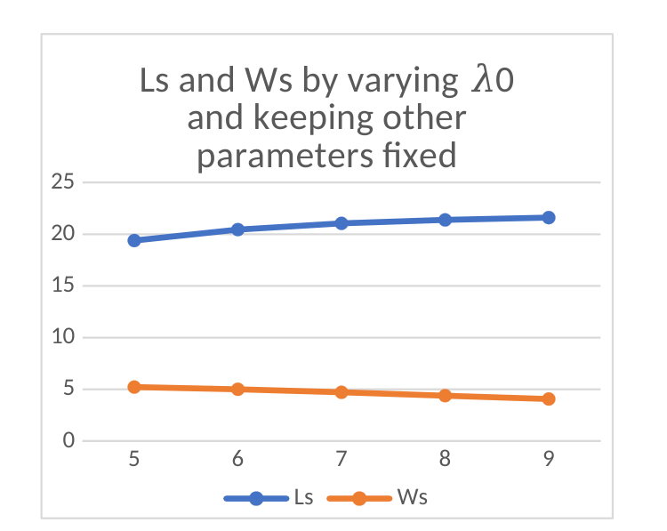
Figure.1: (Finding Ls and Ws by varying 𝜆0 and keeping other parameters fixed)

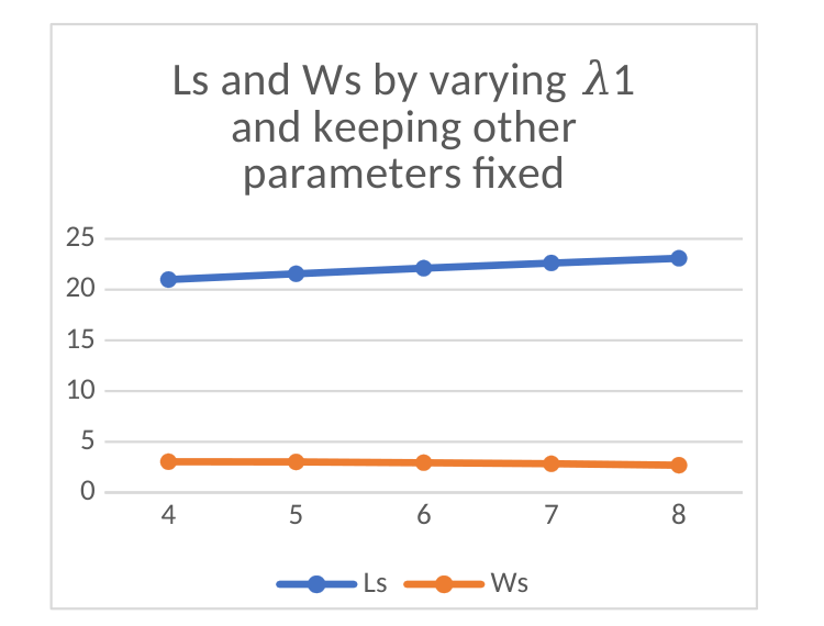
Figure.2: (Finding Ls and Ws by varying 𝜆1 and keeping other parameters fixed)

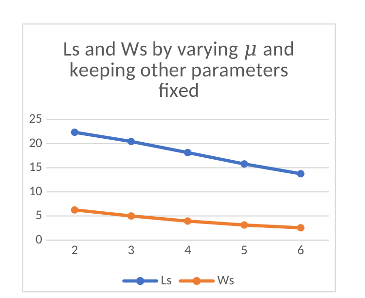
Figure.3: (Finding Ls and Ws by varying 𝜇 and keeping other parameters fixed)

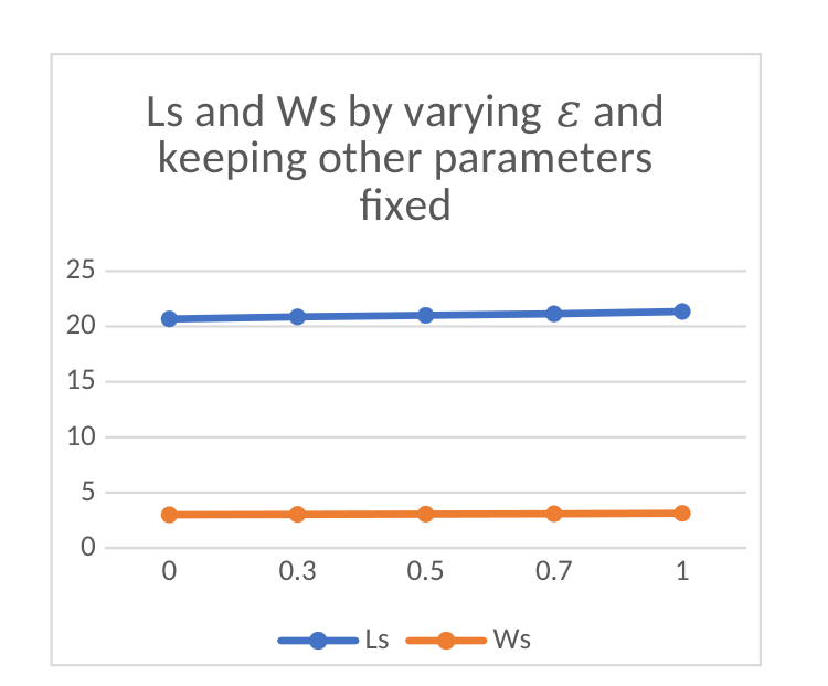
Figure.4: (Finding Ls and Ws by varying 𝜀 and keeping other parameters fixed)

Table 2: When c=2

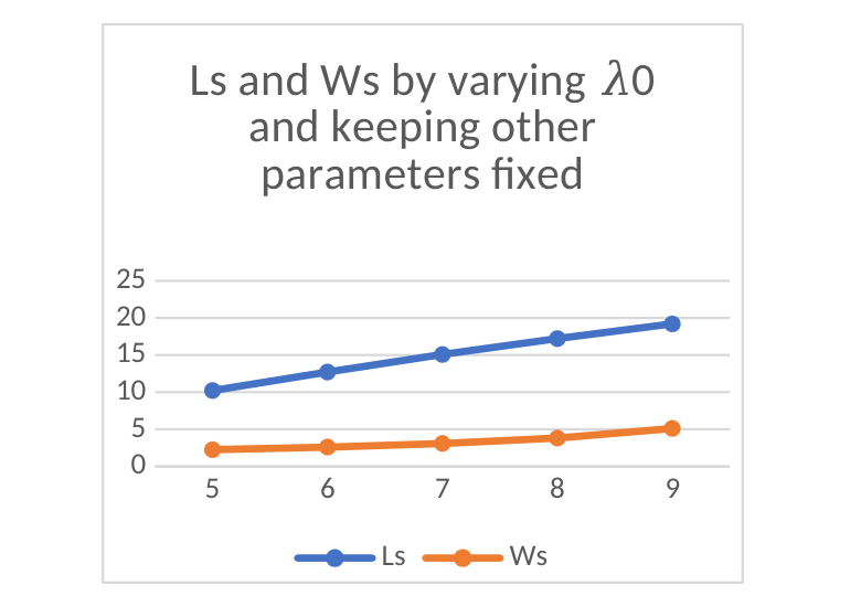
Figure.5: (Finding Ls and Ws by varying 𝜆0 and keeping other parameters fixed)

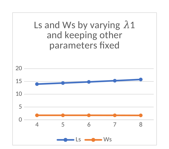
Figure.6: (Finding Ls and Ws by varying 𝜆1 and keeping other parameters fixed)

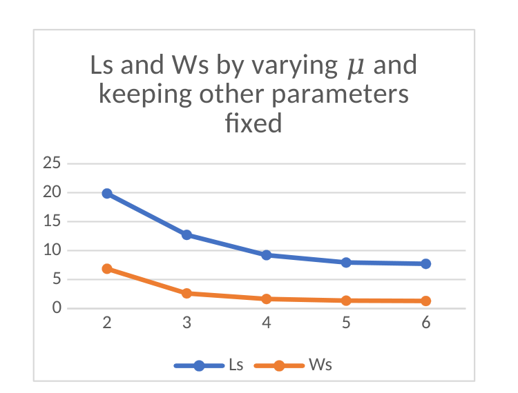
Figure.7: (Finding Ls and Ws by varying 𝜇 and keeping other parameters fixed)

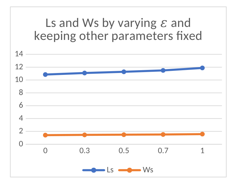
Figure.8: (Finding Ls and Ws by varying 𝜀 and keeping other parameters fixed)

6. Conclusion

The reported tables show that increasing the service rate, with the other parameters fixed, decreases both Ls and Ws. Increasing the dependence parameter epsilon increases both quantities in the displayed examples. Increasing the number of parallel servers generally reduces Ls and Ws in these examples, although the c=2 waiting time exceeds the c=1 value for the row with lambda0=6, lambda1=2, mu=2 and epsilon=0. Increasing an arrival rate increases Ls in the displayed examples; the direction of the change in Ws depends on the arrival-rate parameter and server configuration. These observations describe the reported numerical tables and do not resolve the model and stability issues identified in the accompanying review.

This paper incorporates the original models as special cases. For instance, when v=0 this model narrows down to the M/M/c/∞ interdependent queuing model that allows for varying arrival rates [1]. When $\lambda_{0}$ tends to $\lambda_{1}$ and $\varepsilon = 0,$ this model shrinks to the M/M/c/∞ queueing system’s analysis using vacations [5]. When $\lambda_{0}$ tends to $\lambda_{1}$,$\ \varepsilon = 0$ and $v = 0$, this model narrows down to the conventional M/M/c/∞ queueing model.

Data Availability Statement

Not Applicable

Funding

No fund received for this project

Conflicts Of Interest

The authors declare that they have no conflict of interest.

EthICAl Approval And Human Participation

No ethics approval is required.

References

1. MI Begum and D Maheswari, The m/m/c interdependent queueing model with controllable arrival rates, Opsearch 39 (2002), no. 2, 89–110.

2. K Srinivasa Rao, T Shobha, and P Srinivasa Rao, The m/m/1 interdependent queueing model with controllable arrival rates, Opsearch 37 (2000), no. 1, 14–24.

3. Yonatan Levy and Uri Yechiali, An m/m/s queue with servers vacations, INFOR: Information Systems and Operational Research 14 (1976), no. 2, 153–163.

4. Eitan Altman and Uri Yechiali, Analysis of customers impatience in queues with server vacations, Queueing systems 52 (2006), no. 4, 261–279.

5. Dequan Yue, Wuyi Yue, and Guoxi Zhao, Analysis of an m/m/c queueing system with impatient customers and synchronous vacations, Journal of Applied Mathematics 2014 (2014)

Cite This Work

To export a reference to this article please select a referencing stye below: