
Abstract
The intervention of Machine Learning (ML) techniques is inevitable, as almost all walks of life have been observing its power and significance. The field of healthcare and medical science have all the more reason to promote the effectuation of ML algorithms. Out of various sub-domains of Artificial Intelligence (AI), the models developed using ML algorithms have been implemented widely at present. Based on the clinical data, ML algorithms help to perform classification of the patients’ status of suffering from a disease or not. There are many ML algorithms available and being used for various experiments on different kinds of data set, as they provide different outcomes with desirable metrics. Implementation of such algorithms not only allow to detect the current status, but also the possibility of a patient having a specific disease or symptoms that would lead to severe conditions in future. Apart from the algorithms, the sample collection methodology and the correct attribute selection is also very important for the purpose. The presented work focuses to devise a model that classify the patient’s status to predict accurately whether a patient is suffering from cardiovascular diseases or is fit, using dimensionality reduction with Artificial Neural Network. A multilayer perceptron model (MLP) on top of principal component analysis (PCA) technique is being implemented. The proposed work has put emphasis on the significant effect of PCA in enhancing the throughput of the ANN and that model proposed here, produces super accurate results on multiple datasets.
Keywords: Artificial Intelligence, Artificial Neural Network, Cardiovascular Disease Detection; Dimensionality Reduction; Deep Learning
Introduction
Heart is amongst the most important body organs that makes the body of a human to perform all other functions. To understand broadly, pumping the blood is the only task performed by this organ but in fact it eventually helps to circulate all the necessary supplies to other body parts like nutrients and oxygen [1]. The pulmonary veins take the oxygen-rich blood from the lungs and help it to reach the heart, where it travels to the left atrium and to the left ventricle as well. Blood enters the aorta as a result of the left ventricle’s muscles contracting. During contraction, the mitral valve stops blood from returning to the left atrium. From the aorta, several arteries diverge, supplying blood to the other organs of the body. Blood that has no or very less oxygen (as it gets consumed by various body parts) drains from the human body into the superior and then the inferior vena cava and then passes via the tricuspid valve in the right atrium through the right ventricle. Oxygen-poor blood travels through pulmonary valve and reaches pulmonary arteries, moving finally to the lungs to receive oxygen from contraction of the right ventricle [1,2]. Plus, blood delivers carbon dioxide to the lungs so that an individual can exhale it. The right direction of blood flow is maintained by valves inside the heart. The tissue that builds up the heart is composed of many layers. The circulatory system is at its centre. A networked system of blood vessels, including the arteries, the veins, and the capillaries, are comprised in this system, which transports blood Figure 1, to and from every part of the human body. Heartbeat’s rhythm and rate of heartbeats are controlled by an electrical system inside the human heart. The proper amount of blood is delivered to the body at the proper rate by a healthy heart. If the heart becomes weak due to illness or trauma, the organs won’t function normally as they don’t receive sufficient amount of blood required [2] any form of heart problem or heart related disease could result in that. With 17.9 million deaths per year, heart
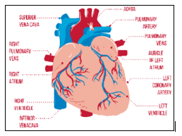
Figure 1: Anatomy of Human Heart
related diseases also known as the cardiovascular diseases (CVDs), contributes to the major cause of deaths around the globe [3]. The cerebrovascular disease, the coronary heart disease, the rheumatic heart disease and other such illnesses are among the different classes of heart related and blood vessel disorders collectively termed as CVDs. Heart attacks and heart-strokes account for more than 4 out of every 5 deaths caused by CVDs, and 1 out of these 3 CVDs deaths come off before the age of 70 years [3]. Premature deaths of such patients can be avoided by identifying the illness in early stages for those who are at high-level risk for CVDs and making sure that they are provided with proper treatment.
To make sure that people in need receive timely care and counselling, access to necessary medications and other fundamental health related technological aids, is crucial and that is where Machine Learning (ML)comes into play. Making the programs and machines Artificial Intelligence (AI) enabled is bound to produce positive results. Whether we talk about prediction of diseases at an early stage or with higher accuracy, ML algorithms answers both of these queries [4]. Detection of various types of diseases can easily and promptly be detected or predicted as per need, the with help of various ML tools and techniques [5-12]. ML algorithms are quite well suited for the processing over the medical datasets. The various machine learning sub-domains are well versed when it comes to such kind of implementations, it has never let down the community.
The Machine Learning domain is broadly categorized into four categories, as follows:
Supervised learning: A kind of machine learning called supervised learning uses labelled data to train an algorithm. Using examples of the right input-output pairings, this method teaches the algorithm how to map inputs (also known as features) to outputs. The training and the testing set of data are generally two components of the labelled data. The validation set is used to assess the algorithm’s performance on untrained data, whereas the other part, the training set is used for training the algorithm. The aim of supervised learning mechanism is to define a function that correctly forecasts the outcome for unknown inputs that have never been seen by the algorithm. Classification and regression are only a couple of the many tasks that supervised learning may be utilized for. In classification, the objective is to predict a discrete output variable from input data, such as the existence or absence of a specific condition. Regression is the process of using input factors to make predictions about a continuous output variable, such as the cost of a house. The Decision-Trees (DTs), the Logistic Regressors (LRs), the Support-Vector Machines (SVMs) and the Neural Networks (NNs) are some popular examples of the supervised learning techniques. These algorithms vary in terms of complexity, effectiveness, and applicability for various kinds of data. Overall, supervised learning is a potent and popular machine learning strategy that enables the development of precise and trustworthy prediction models for a range of applications.
Unsupervised learning: Unsupervised learning technique is listed under the domain of machine learning, which deals in the algorithms that discover links and patterns in a given dataset without having access to the output or labels beforehand. So, when a dataset lacks any predetermined target variables or target class names required for the algorithm to predict, unsupervised learning is used. Finding hidden structures, correlations, or patterns in the data is the aim of unsupervised learning. This is accomplished by analyzing the data using statistical methods and functions to find patterns or distinctions between various data points. One of the methods most frequently employed in unsupervised learning is clustering. Based on their characteristics or traits, clustering algorithms bring together related data items. Clustering, for instance, is suitable for making groups of clients according to their purchasing patterns or photographs according to visual similarities. Dimensionality reduction is a frequent method used in unsupervised learning. To minimize the count of features or independent variables used in the available data while keeping the most crucial data, dimensionality reduction strategies are implemented. When working on datasets having a large number of dimensions, where it could be challenging to visualize or analyze the data, this might be helpful. However, because there is no rule of thumb or right response to direct the algorithm, it may be more difficult than supervised learning. In order to get meaningful results from unsupervised learning, careful preparation and algorithm adjustment are necessary because here the model detects and groups the data points based on their features and associated values, as done in case of algorithms like k-means clustering, DBSCAN, Principal Component Analysis (PCA) etc.
Reinforcement learning: A branch of artificial intelligence called reinforcement learning is concerned with how an agent might learn to choose actions that will minimize or maximize a predefined numerical penalty or reward metric. In this machine learning technique where the agent interacts with the surroundings and gains knowledge through the penalty as well as rewards it gets. The reinforcement learning agent is envisioned as a system that performs decision-making tasks in order to interact with the environment in accordance with its present state and receives the feedbacks from environment, it is acting inside, in form of rewards or penalties. The objective of the agent is mainly to discover a policy or a kind of mapping between states and action that helps to maximize the overall reward at the end. Examples of commonly used reinforcement learning algorithms are namely the Q-learning mechanism, the State-Action-Reward-State-Action (SARSA) algorithm etc.
Deep learning: The Deep learning mechanism is a type of machine learning approach that uses multiple-layered ANNs to simulate intricate connections between the provided input and the output thus generated. Deep learning algorithms are especially helpful for applications like natural language processing, audio recognition, image recognition and autonomous systems because they can handle vast volumes of data and automatically extract pertinent characteristics from raw data. The utilization of deep neural networks, which include numerous layers of linked nodes and each layer is in charge of learning a distinct element of the input data, is the core component of deep learning. The network’s initial layer takes the raw input data, and later layers extract higher-level features using the features that had been learnt by earlier levels. The weights of the nodes as well as the biases of the network are changed throughout the training of a deep learning model so that the discrepancy between the expected output and the actual output can be reduced. This is often accomplished using a form of stochastic gradient descent. Until the model achieves an acceptable degree of accuracy, the procedure is repeated over a number of iterations. The Convolutional Neural Nets (CNNs), the Multilayer perceptron, the Recurrent Neural Nets (RNNs) are few commonly used examples of the deep learning mechanism. These designs are suitable for various jobs and have diverse characteristics.
In the presented work, we have used and experimented over various supervised learning techniques followed by Bagging and Boosting algorithms besides a Multilayer Perceptron model for classification of CVDs as per recorded data of patients, taken at the Cleveland, the Hungary, the Switzerland, and the VA Long Beach medical facilities and stored on the Kaggle’s website [13,14]. The two main techniques emphasized in the presented work are PCA and MLP models.
PCA, an unsupervised ML technique as well as a statistical technique, is used to find trends and connections in a dataset. It is a method used in pattern recognition, machine learning, and data analysis to simplify a dataset while retaining as much crucial data as feasible. Finding the directions of highest variance in the data allows PCA to determine the underlying pattern in the dataset. In other words, it is a technique that reduces the complexity by decreasing the number of dimensions in a dataset with high dimensionality by locating its most crucial properties. The direction with the highest variance in the dataset is represented through the first selected principal component and following components are orthogonal to the first and have the maximum possible variance within that constraint. The data is transformed linearly to produce these components, which groups the independent variables present in the original dataset into a separate collection of variables known as primary components. PCA is frequently applied to data compression, data visualization, and exploratory data analysis. It may be simpler to see and interpret the data by lowering its dimensionality. By minimizing the noise and redundancy in the data, PCA plays a very important role for other machine learning techniques, such clustering and classification.
Talking about other techniques, an MLP model is comprised of numerous layers each having linked nodes, or what is known as neurons. A mathematical function, each neuron executes a weighted sum of its input values, followed by a nonlinear activation function. After that neurons present in the next layer receive each neuron’s output as input. While the output layer of an MLP creates the network’s ultimate output, the input layer, designed to initiate the process, of an MLP is made up of neurons that take input data. The majority of the computational activity is located in the hidden layers, which are levels that are situated in between the two layers, one on either side, namely the input and the output layer. To get the desired output from an MLP, it must be fed with input data and then the corresponding weights of the connections must be changed amongst the neurons present in each layer. Backpropagation, a technique commonly used for this, includes calculation of the error between the network’s predicted output and the actual produced output, then modifying the weights metric to reduce the error. MLPs are often used in machine learning and may be utilized for many different tasks including speech recognition, picture recognition and other complex tasks.
The presented work is focused to establish and advocate an innovative approach for the use of a combination of supervised and unsupervised ML algorithms, for detection of cardiovascular diseases / heart diseases in the patients in order to save millions of lives.
Literature Review
The presented work is backed by study of literature in related domain, where ML as a worthy sub-domain of AI has proved its worth in the field of medical science [4-12].
Out of various classes of cardiovascular diseases, some are very significant. As per the structure of the organ, the major reason is the lack of uniformity of the flow of the blood through the system. Unhealthy habits of eating, inactivity for longer time periods, frequent usage of tobacco products and by-products, and regular abusive use of alcohol are the prime behavioural risk factors for CVDs [1-3]. One may observe high blood pressure, high level of blood glucose, high readings for blood lipids, as well as obesity as a result. Such “intermediate risk variables” can be easily estimated at the primary healthcare centers and intimated to the patients about their high risk of resulting in serious CVDs. Various scientists have devised multiple way outs, even in the field of AI, multiple sub-domains have been explored for the same [15-19]. From Fuzzy models to Neural Networks and Deep Learning tools as well have been suggested in various works by analysts and researchers. Out of all these implementations, Machine Learning models have shown a very good response in diagnosis of diseases at early stages to save large number of lives [20-21].
Heart related diseases have appeared as a big contributor in case of death tolls all over the globe in past years. There are mainly 4 categories of the patients complaining about heart related issues. Symptoms were based on the exposure of physical activities and discomfort therewith [22-24]. A comparative study of the referred texts is presented below in Table 1.
Table 1:Comparative Analysis of Literature
| Ref. | Methodology | Datasets | Findings | Remarks / Research Gap |
| [4] | LR Classifier, NB Classifier, SVM Classifier | Wisconsin Diagnostic Breast Cancer Dataset | Accuracy, precision, recall, f1-score | Simple and effective, but work done on only a single dataset; For Breast Cancer |
| [6] | NBC, SVM, Bi-clustering and AdaBoost, RCNN, Bidirectional RNN | MGCHRI, India Dataset | Accuracy, precision, recall | For Breast Cancer Detection; Based on image processing; Design complexity |
| [12] | Decision Tree(DT), Gradient Boosting, RF, MLP, NB, LR | Heart Disease Dataset – UCI | Accuracy, f1-score, recall | Excellent results, but only able to perform the classification on Cleveland and Hungry datasets |
| [21] | Ensemble technique (K nearest neighbor, RF, DT) | Heart disease Dataset – UCI | Accuracy, f1-score, precision | Multiple techniques use, but lesser accuracy as compared to our work |
| [22] | RF, NB, DT, SVM classifier | UCI Heart disease Dataset | Accuracy | Simple and straight-forward implementation. Lesser accuracy as compared to our work |
| [27] | Feature Scaling, SVM classifier | Wisconsin Diagnostic Breast Cancer Dataset | Accuracy | Small dataset; Single Dataset; Emphasis on only on technique |
| [29] | Ensemble Technique (SVM, NB, RF, DT, LR) | UCI Heart disease Dataset | Accuracy | A variety of techniques were used, but attained lesser accuracy as compared to our work |
| [30] | K-means, Outlier Detection | Kaggle Healthcare Fraud Detection database | F1-score,Accuracy, AUC | The work was focused on unsupervised technique; Overall performance by the proposed model is good |
| [31] | ExtraTrees, Lightgbm, SGDC, Nu SVM, Adaboost, XGBoost and Gradient Boosting | UCI Heart disease Dataset | F1-score,Accuracy, AUC | A variety of techniques were used, but attained lesser accuracy as compared to our work |
| [32] | DT, NB, K-NN, RF | UCI Heart disease Dataset | Accuracy | Very simple and direct implementation of ML techniques; lesser accuracy as compared to our work |
| [34] | LR, NB, SVM, KNN, DT, RF, ANN, DNN, MLP | UCI Heart disease Dataset | Accuracy | The work is comprised of a comparative analysis of a bunch of ML Techniques, but none of them surpassed the accuracy achieved by the model proposed in our work |
| [35] | DT, SVM, NB, LR, RF | Samples collected from KT Hospital and Lady Reading Hospital, Pakistan | Accuracy | Experiments were carried out on a firsthand collected samples and various ML techniques were used, but attained lesser accuracy as compared to our work in all cases |
| [37] | DT, RF, NB, K-Nearest Neighbor, LR, And SVM | UCI Heart disease Dataset | Accuracy and f1-score | A variety of techniques were used by the author |
A lot of studies referring to heart disease detection using ML techniques are done in past. Many researchers have tried different tools, techniques and algorithms for the fulfillment of their objectives. Out of which several algorithms received higher accuracy, while a few scored comparatively low with same or other algorithms [25-36]. The work presented in the paper has a chosen set of ML algorithms to perform the prediction for the case of heart related disease in patients. This paper targets to solidify the notion of implementation of ML algorithms in the field of healthcare and medical science [37-45]. After going through the various works done by different researchers on various algorithms, we picked up a set of selected algorithms to find and establish the feasibility for predicting the status of organ inefficiency in early stages of heart related disease.
This paper, thus deals in the area of finding the better performance of ML algorithms by implementing parallel and complementing techniques, as well as to focus the importance of other significant metrics such as sensitivity or precision, recall etc. to make double sure that the model proposed works fine enough when predicting targets for unknown dataset. A handful of concepts related to different machine learning techniques were studied and experimented over to make sure the selected algorithm or set of algorithms fit properly and produce favorable output during the final prediction on the patient’s records.
Dataset
In this paper, experiments were carried out on two datasets based on the Cleveland, Hungary, Switzerland, Long Beach combined, that we have used by the name Dataset-1[13] and Dataset-2[14]. Out of these two datasets, Dataset-1 had total 75 features as recorded, but later on analysts found over time, that 14 of them are the most useful and thus the processed dataset contains the selected features only. The other one consists of a total of 12 features. During the preprocessing stage, the dataset has been checked for discrepancies (if any). For example, we checked for the correlation amongst all features and the heatmap is presented as Figure 2 and Figure 3.
The Dataset-1 contains various measures recorded from the patients, significant of all, the following features are considered for the final set of data for experiments: –
age: patient’s age.
sex: patient’s gender.
cp: type of chest-pain.
trestbps: reading of blood pressure in rest.
chol: level of cholesterol.
fbs: blood-sugar level during fast.
restecg: ECG readings during rest.
thalach: max. reading for heartbeat.
exang: exercise causing angina in patient.
oldpeak: ST depression due to exercise / rest.
slope: ST segment peak exercise slope.
ca: no. of major vessels colored during fluoroscopy.
thal: probably thalassemia, no details given.
target: the output class for prediction.
The target feature is used as the output class for prediction of heart disease in the presented work. The field holds a value ‘0’ to represent ‘No Heart disease’ or value ‘1’ to represent heart disease in order to perform binary classification. However, in the original dataset the target field was named as “num” and held values = {0,1,2,3,4} to represent the patient status as follows: –
0 = No risk of heart disease
{1,2,3,4} = different categories of heart disease
The values then transformed for binary classification during the data preprocessing stage.
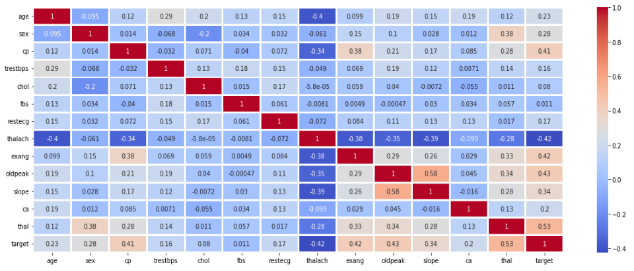
Figure 2:Heatmap of correlation of the dimensions in the Dataset-1
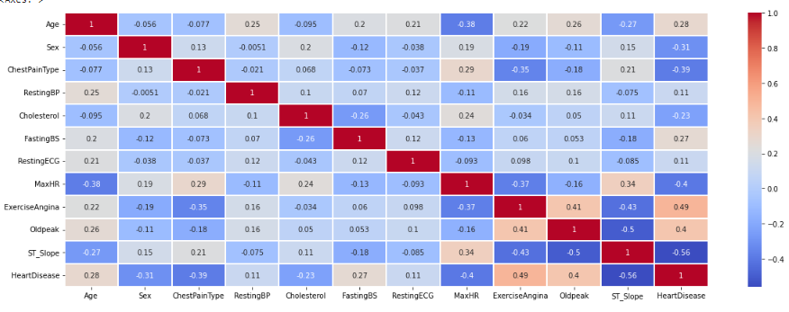
Figure 3: Heatmap of correlation of the dimensions in the Dataset-2
The Dataset-2 is comprised of a total of 12 features as follows: –
Age (ranging from 27 years to 77years)
Sex (Male and Female)
ChestPainType (ASY, ATA, NAP, TA)
RestingBP (as per reading)
Cholesterol (as per reading)
FastingBS (Y/N)
RestingECG (LVH, Normal, ST)
MaxHR (as per reading)
ExcerciseAngina(Y/N)
Oldpeak (as per reading)
ST_Slope (Down, Flat, Up)
HeartDisease (Y/N)
These features are basically extracted from the original and unprocessed dataset from the medical facilities of Cleveland, Long Beach, VA and Switzerland but with reduced dimensions and different set of records as compared to the Dataset-1. Further both the datasets have been processed for desired features before experimenting with the proposed model. Data-preprocessing methods used in the presented work are addressed further in the following section.
Methodology
The presented work focuses on the notion of using ML tools and techniques to predict heart disease risk in a patient. Various experiments have been done in related field, for different disease categories at different stages of infection, more or less aimed to promote the implementation of ML algorithms for all plausible applications in the field of healthcare and medical science. The workflow of proposed model is depicted here Figure 4. First of all, the dataset [13] was selected for the experiment and then all required preprocessing tasks were carried out. To name a few, missing data records were identified and removed, some values and datatypes were transformed to suit the nature of experiments viz. the feature “ca” and the feature “thal” were defined in the original dataset as object type, which were then transformed into “float64” datatype of Python environment, without any loss of data. The feature “target” having multiple output classes was then dealt with and all different heart diseases categories were consolidated as one single category to be represented by “1” while the no disease category remains same and represented by “0”.
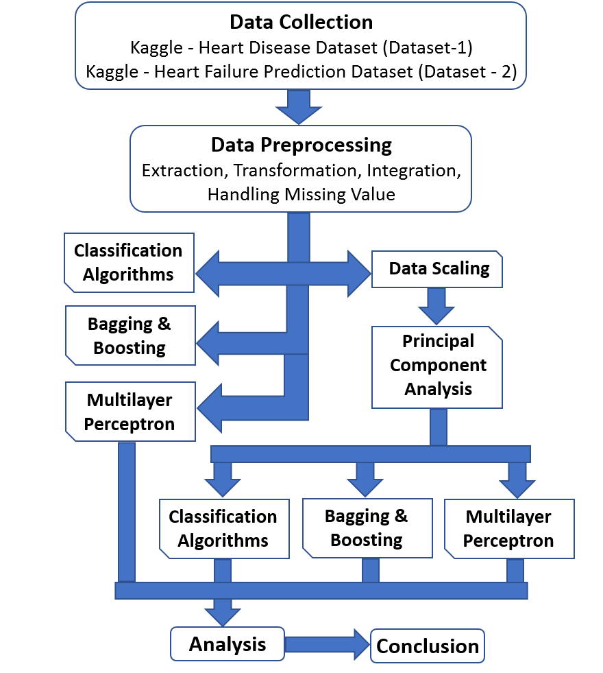
Figure 4: Workflow of the proposed model
Similarly, Dataset-2 was also prepared for the experiments and for further comparative analysis before drawing any conclusion. Features like, “ChestPainType”, “RestingECG”, “ST_Slope” were having non-numeric values those were categorized and transformed to be used for the implementation of ML algorithms. Initially, only twelve features were extracted from the set of a large number of unimportant features and also the missing values from the recorded dataset were simply removed, so that they could not offer any deviation from the attempted estimations with high accuracy.
Further working on the correlation and other obvious measures, the task of data preprocessing was finished. The next step was to prepare data frames for the various algorithms. Using the “sklearn” library of Python, the training and the testing data frames were created in the ration of 75:25 with a “random state” value 10 units for both the datasets. Multiple algorithms were then tested, over the so data frames so obtained, one after the other. In order to enhance the prediction of the output class, bagging and boosting techniques were implemented in form of the Random Forest algorithms and the Adaptive Boosting (AdaBoost) algorithm respectively and a Multilayer Perceptron model was also used on both the datasets.
As represented in the Figure 4, the workflow is comprised of two separate ways of implementing these algorithms over the datasets. A special emphasis was to observe the effect of using the Principal Component Analysis technique before using the supervised ML algorithms for classification of data. The algorithms were synthesized with various combinations of parameters and optimum value has been included for the next stage, i.e. the comparative analysis of accuracies, precision and similar measures for a final verdict of the predicted outcome After the preprocessing stage was completed, the “countplot” was created for the output class Figure 5 & Figure 6 . The count of patients recorded for No-disease category is represented by output class “0” and that of for the Disease category is the output class “1” .
Using the pandas, numpy, sklearn, pyplot and seaborn libraries of Python, all the experiments were carried out. Various classification and ensemble modules were used for the purpose. Different charts were rendered to visualize the significance of various features over the output data, as Figure 7 & Figure 8 represent the distribution of “age” feature against the output classes “Disease” (1) and “No-disease” (0).
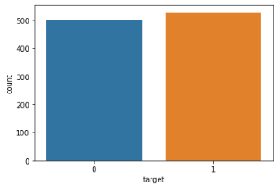
Figure 5: Disease (1) – No-disease (0) count for Dataset-1
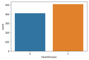
Figure 5: Disease (1) – No-disease (0) count for Dataset-2
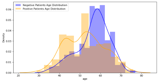
Figure 6: Age distribution for “Disease” and “No-disease” Dataset-1
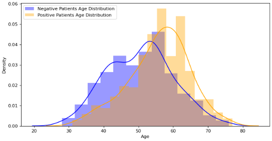
Figure 7: Age distribution for “Disease” and “No-disease” Dataset-2
Broadly speaking, the patients of age range between 45 -55 years in Dataset-1 and age range[50,65] in Dataset-2 were seen to be suffering the most with CVDs as shown in Fig. 5(a) & Fig. 5(b) respectively.. Both datasets were prepared for similar statistical renders for a broader overview on different features. While working on Dataset-2, feature transformation was a major processing task as a number of features were comprising of data not suitable for numerical models. At the same time many records with missing or unknown values were removed.
Further, the model was trained with 75% of the data separately from both the datasets and the remaining were kept for the purpose of testing. Usually an 80:20 ratio is used for the split purpose, here in the presented work we kept the bar a little high and worked with comparatively less trained model to identify the actual capability of the model. Once the different algorithms predicted the target values, a detailed comparison was carried out not only on the basis of the accuracy score but drilling down into the various metrics for the effectiveness of the proposed model. A total of six different algorithms were used to reach the final conclusion and at each step we found the increasing accuracy of the experimented models. We worked on SVM classifier, LR Classifier, NB Classifier, RF Classifier, Adaptive Boosting – SAMME and a Multilayer Perceptron model at last. Another aspect, the presented work focused on, was the use of scaled data and implementation of Principal Component Analysis on each of the algorithms one-by-one. The idea was to formulate an effective combination of supervised and unsupervised ML techniques for a better result while making predictions.
The dimensionality reduction mechanism is implemented with help of the Principal Component Analysis (PCA) technique. It was found that, after reduction in dimensionality the performance of the various algorithm fluctuated in both positive as well as negative direction. The reduction in dimensionality improved the overall performance and the execution time. And the best algorithm thus selected after implementation of PCA and averaging the attained accuracy over both datasets.
PCA is used here to transform the set of potentially correlated features into uncorrelated features termed as the principal components as per the following steps:
Data Centering is done first by subtracting the mean from each variable to center the data around the origin. Say, X be the centered data matrix with dimensions n x p, where n represents the no. of observations while p is the no. of variables.
Covariance Matrix C is computed of the centered data matrix X. This covariance matrix C is a symmetric p x p matrix, where the element in the row no. i and column no. j is the covariance between the i-th & j-th variables. Covariance between 2 variables xi and xj can be calculated as:
(1)
where the summation is over all n observations.
Eigenvalue decomposition is done after that, on the covariance matrix C. Here matrix C can be decomposed as C = VDV^T, where V is a p x p matrix of eigenvectors and D represents a diagonal matrix of the same. So, the eigenvectors in V represent the directions of the principal components and the corresponding eigenvalues in D represent the amount of variance explained by each principal component.
Principal Components are then selected as a subset of the eigenvectors based on the desired number of dimensions or the amount of variance explained. Let k be the desired number of principal components. Choose the k eigenvectors representing the k largest values. Let P be a matrix of dimension p x k, consisting of these selected eigenvectors.
Dimensionality Reduction is done finally by projecting the centered data matrix X onto the selected principal components. The transformed matrix Y is obtained as Y = XP, where Y has dimensions n x k. This resulting transformed data matrix Y contains the principal components, which are uncorrelated variables that capture the most significant variation in the original data.
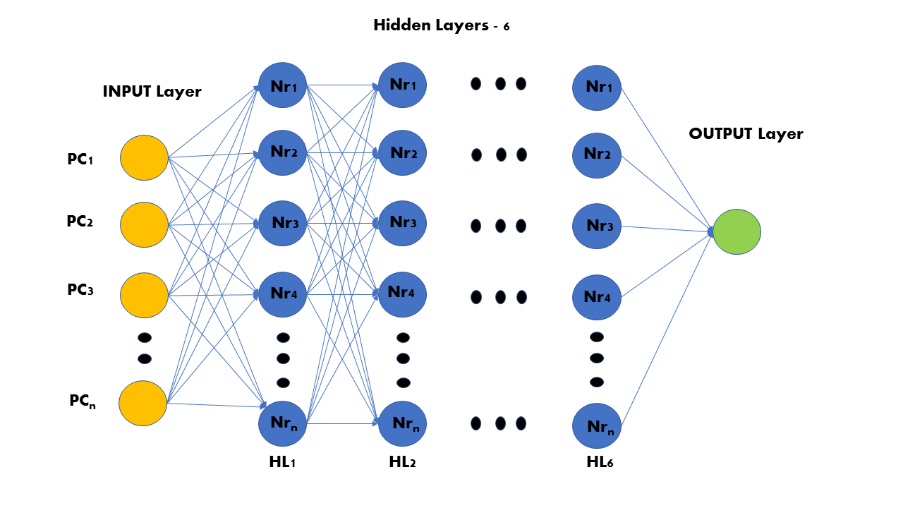
Figure 8: Multilayer Perceptron model
Further, an MLP model is used as an ANN with 8 layers, including an input layer, 6 hidden layers having an optimized number of neurons, and the output layer Fig. 6 . Input to network’s fit () function is denoted as xtrain and ytrain. The MLP works as follows:
Weighted input is calculated first of all. For each neuron j in layer l, the weighted input is calculated by taking a weighted sum of the outputs of the previous layer (l-1) and adding a bias term represented as:
(2)
where w_ij^l represents the weight between neuron I in layer (l-1) and neuron j in layer l, a_i^(l-1) is the output of neuron I in layer (l-1), and b_j^l is the bias term for neuron j in layer l.
Activation Function is then implemented, our model uses the default Rectified Linear Unit (ReLU) function. Here the weighted input is passed through the ReLU activation function to introduce non-linearity. Other available and common activation functions include sigmoid, tanh and softmax, but the performance of the ReLU function was found optimum in this case. The processed output of the activation function thus used, is denoted as a_j^l. Thus, we represent the relation between the input and the output produced as follows:
(3)
where f is the chosen activation function.
The next step is called the ‘Forward Propagation’ in which the outputs of each layer from the input to the output layer is computed. It is represented as follows:
For the input layer (l = 0):
(4)
For hidden layers (1 ≤ l ≤ L-2):
(5)
(6)
For the output layer (l = L-1):
(7)
(8)
Next, we measured the difference of predicted output (a_j^(L-1)) i.e., ytest and the true output (ypred). The loss function depends on the specific problem being solved, here we used the default Mean Square Error (MSE) function for the proposed model.
Finally, the ‘Backpropagation’ is utilised to update weights & biases to minimize the loss function. It involves calculating the gradients of the loss function w.r.t. weights & biases and using the gradient descent algorithm to update the parameters.
On the basis of the above-mentioned method, proposed algorithm is presented as Algorithm 1, below.
Algorithm 1
Input: Heart_Disease.csv as dataset_1, Heart_Failure_Prediction.csv as dataset_2
Output: Heart Disease prediction algorithm
Begin
Read Heart_Disease.csv as dataset_1, Heart_Failure_Prediction.csv as dataset_2, r1[ ] as empty, r2[ ] as empty, pro_algo as empty, avg_accuracy = 0 , max_accuracy = 0
Clean dataset_1, dataset_2
Check for correlations
Transform the dataset_1, dataset_2
Delete and fill unknown and missing value
Spilt dataset_1, dataset_2 in trainset and testset
Prepare scaled data through StandardScaler ()
Fit the model using PCA ()
For I in range (1, 2)
Call SVC (), Insert svc_acc at ri [1]
Call NBC (), Insert nbc_acc at ri [2]
Call LRC (), Insert lrc_acc at ri [3]
Call Random_Forest (), Insert rfc_acc at ri [4]
Call Ada_Boost (), Insert nbc_acc at ri [5]
Call MLP (), Insert lrc_acc at ri [6]
End For
For i in range (1 ,6)
avg_accuracy = (r1[i]+r2[i]) / 2
If avg_accuracy is greater than max_accuracy
Then max_accuracy = avg_accuracy
End For
Update the best algorithm having max_accuracy
End
ANALYSIS & DISCUSSIONS
Various algorithms and their parameters in various combinations yield result on the given datasets. As represented below, Table 2 and Table 3 represents the attained accuracy of proposed model is highest at 86% for Dataset-1 and 99% for Dataset-2.
For Dataset-1, the SVC model, the NBC model, the Random Forest classifier and the MLP model attains the highest accuracy overall. The NBC model and the Random classifier model attained the highest accuracy of 84% without PCA same as the MLP model, while the MLP classifier attained the same highest accuracy of 86% upon PCA as shown in Table 2.
For Dataset-2, the MLP classifier attained the highest value for accuracy of 99% amongst all algorithms. The RF classifier attained highest accuracy metric without using PCA, while the MLP model attained the highest value for accuracy after implementation of the PCA technique as depicted in Table 3.
Table 2: Results on Dataset-1
| Comparative Analysis of accuracy for Dataset-1 | ||
| Classifiers | Accuracy (without PCA) | Accuracy (with PCA) |
| SVC | 0.70 | 0.84 |
| NB | 0.84 | 0.83 |
| LR | 0.83 | 0.83 |
| Random Forest | 0.84 | 0.83 |
| AdaBoost | 0.82 | 0.81 |
| MLP | 0.84 | 0.86 |
Table 3: Results on Dataset-2
| Comparative Analysis of accuracy for Dataset-2 | ||
| Classifiers | Accuracy (without PCA) | Accuracy (with PCA) |
| SVC | 0.70 | 0.91 |
| NB | 0.84 | 0.84 |
| LR | 0.87 | 0.87 |
| Random Forest | 0.97 | 0.97 |
| AdaBoost | 0.86 | 0.80 |
| MLP | 0.85 | 0.99 |
The most interesting observation is the improvement in performance of the Multilayer Perceptron model upon implementation of the Principal Component Analysis technique. In both the datasets, it is clearly seen that there is a very positive significant change in the attained value of accuracy.
Table 4: Finding the best algorithm for the model
| Cumulative Analysis of accuracies for Dataset-1 and Dataset-2 | |||
| Classifiers | Accuracy (D1 – with PCA) | Accuracy (D2 – with PCA) | Avg. of Accuracies (Max accuracy) |
| SVC | 0.84 | 0.91 | 0.88 |
| NB | 0.83 | 0.84 | 0.84 |
| LR | 0.83 | 0.87 | 0.85 |
| Random Forest | 0.83 | 0.97 | 0.90 |
| AdaBoost | 0.81 | 0.80 | 0.81 |
| MLP | 0.86 | 0.99 | 0.93 |
To analyze the performance of the used algorithms and to decide which works better on varying datasets, we compared the attained accuracies of all algorithms used on both datasets by summing up their values as presented in Table 4. We found that reducing dimensionality of the available data in both the datasets, the model implementing MLP performs the best, with the cumulative average accuracy = 93% termed as the max accuracy of proposed model.
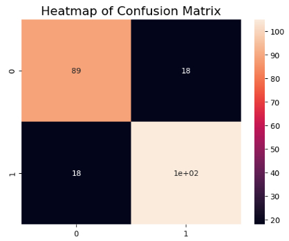
Figure 9: Confusion matrix of MLP model without PCA for Dataset-1
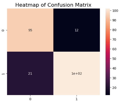
Figure 10: Confusion matrix of MLP model with PCA for Dataset-1
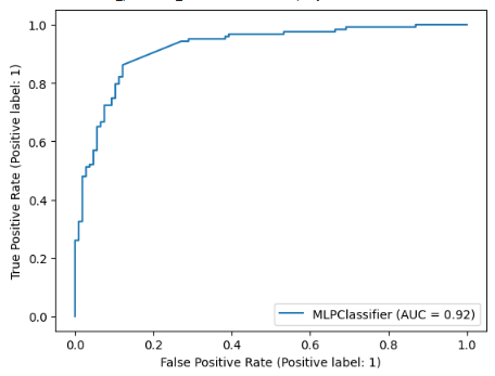
Figure 11: ROC-AUC of MLP model with PCA for Dataset-1
For Dataset-1, the accuracy of the MLP model has increased to 86% from 84%, as shown in Table 2, after PCA integration and for Dataset-2, accuracy has increased from 85% to 99%, as shown in Table 3.
Further, a notable change is observed for the SVC model before and after using the PCA on both datasets. the accuracy of the LR classifier remained same in both cases. Another interesting observation is the slight negative impact of the PCA technique over the NB classifier for Dataset-1, but no change in case of Dataset-2 and the same impact is observed for the Random Forest classifier as well. The adaptive boosting mechanism however reflected only decreased accuracy when implemented with the PCA technique.
The results were verified with corresponding confusion matrixes figure 9 & 10 for Dataset-1. Before and after implementation of the PCA technique, there is a positive change. Now the result has improved and there are predictions with 86% accuracy, which is acceptable. Further, if we consider another metric, Receiver Operating Characteristic (ROC) we find the model working quite well. Area Under the ROC Curve (AUC) plotted in Figure 11 shows that the 92% area is covered under the ROC curve, i.e., the efficacy of the model has a worth to be considered.
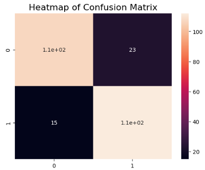
Figure 12: Confusion matrix for MLP model without PCA for Dataset-2
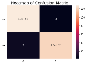
Figure 13: Confusion matrix for MLP model with PCA for Dataset-2
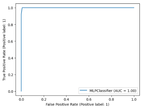
Figure 14: ROC-AUC of MLP model with PCA for Dataset-2
For Dataset-2, the results were similar to that of Dataset-1. As represented in Figure 12 & Figure 13 are the corresponding confusion matrixes for the predictions done by the MLP model before and after the use of PCA over Dataset-2. Implementation of the Principal Component Analysis before using the MLP model brings the accuracy up to over 99% as compared to the previous case where we get from MLP without PCA an accuracy of 85% and more importantly it can make correct predictions almost every time out of hundred patients. Now the result has improved and there are only three (3) FP values and only seven (7) FN values, which is clearly acceptable. The same is depicted with help of the AUC plotted in Figure 14. Here the area under the curve is almost 100%, which nearly to predict the correct value for disease and no-disease every single time, however we highlight the case that with increase in number of patients / data this accuracy needs to be further enhanced.
Therefore, we observe that the proposed PCA integrated MLP model is suitable for making predictions for the patients and promises to save millions of lives with its implementation at medical facilities round the globe. If we talk about the limitations of the presented work, the major is that the datasets used belong to a certain part of the globe only and thus may not represent the other regions and habitats in that well manner. Other than that, we may further try to enhance the accuracy because with even a 99% accuracy in prediction, there will be thousands of cases per million of population wrongly detected. So, we say that definitely the proposed model assists to reduce the risk of death, at the same time further improvements are welcomed.
Conclusion
Machine Learning has evolved as one of the strongest sub-domains of AI for the field of medical science. Different algorithms have proven to aid specific applications to increase the throughput significantly. The presented work adds on to the notion of applying ML algorithm for diagnosing patients having disease that are difficult to be detected in early stages or accurately detected with arrangements available earlier. Thus, we can state that implementing ML tools and techniques are very promising for various mundane tasks as well as the field of medical science. To be specific, out of the several models used for the experiment over different datasets, the Multilayer Perceptron model performed the best upon using the Principal Component Analysis. It is clearly assertible that the ANN model yields very accurate predictions. Thus, we conclude that using innovative ANN models are suitable and effective technique for classification purpose.
References
Britannica – Home – Health & Medicine – Anatomy & Physiology https://www.britannica.com/science/heart
National Heart, Lung and Blood Institute – An official website of the United States government. https://www.nhlbi.nih.gov/health/heart
World Health Organization, Cardiovascular Diseases, WHO, Geneva, Switzerland, 2020, https://www.who.int/healthtopics/cardiovascular-diseases/.
Anshuman and U. Kumar, “Machine Learning model for detection of Breast Cancer,” 2021 IEEE Xplore 5th International Conference on Information Systems and Computer Networks (ISCON), Mathura, India, pp. 1-4
H. A. Esfahani and M. Ghazanfari, “cardiovascular disease detection using a new ensemble classifier,” 2017 IEEE 4th International Conference on Knowledge-Based Engineering and Innovation (KBEI), 2017, pp. 1011-1014.
Anji Reddy Vaka, Badal Soni, Sudheer Reddy K., Heart disease detection by leveraging Machine Learning, ICT Express, Volume 6, Issue 4, 2020, pp. 320-324
Shen, L., Margolies, L.R., Rothstein, J.H. et al. Deep Learning to Improve Breast Cancer Detection on Screening Mammography. Sci Rep 9, 12495 (2019)
S. N. Rao, P. Shenoy M, M. Gopalakrishnan and A. Kiran B, “Applicability of the Cleveland clinic scoring system for the risk prediction of acute kidney injury after cardiac surgery in a South Asian cohort”, Indian Heart J., vol. 70, no. 4, 2018, pp. 533-537
M. S. Amin, Y. K. Chiam and K. D. Varathan, “Identification of significant features and data mining techniques in predicting heart disease”, Telematics Inform., vol. 36, Mar. 2019, pp. 82-93.
S. Shalev-Shwartz and S. Ben-David, “Understanding machine learning,” From Theory to Algorithms, Cambridge University Press, Cambridge, UK, 2020.
R. Chen, N. Sun, X. Chen, M. Yang, and Q. Wu, “Supervised feature selection with a stratified feature weighting method,” IEEE Access, vol. 6, pp. 15087–15098, 2018.
K. Garate-Escamila, A. Hajjam El Hassani, and E. Andr ´ es, ` “Classification models for heart disease prediction using feature selection and PCA,” Informatics in Medicine Unlocked, vol. 19, Article ID 100330, 2020.
Kaggle – Heart Disease Data Set. https://www.kaggle.com/datasets/johnsmith88/heart-disease-dataset?resource=download
Kaggle – Heart Failure Prediction Dataset https://www.kaggle.com/datasets/fedesoriano/heart-failure-prediction
K. Uyar and A. Ilhan, “Diagnosis of heart disease using genetic algorithm based trained recurrent fuzzy neural networks”, Procedia Comput. Sci., vol. 120, 2017, pp. 588-593.
M S. A. Pattekari and A. Parveen, “Prediction System for Heart Disease Using Naive Bayes”, International journal of Advanced Computer and Mathematical Sciences, vol. 3, no. 3, 2012, pp. 294-290.
C.-A. Cheng and H.-W. Chiu, “An artificial neural network model for the evaluation of carotid artery stenting prognosis using a national-wide database”, Proc. 39th Annu. Int. Conf. IEEE Eng. Med. Biol. Soc. (EMBC), Jul. 2017, pp. 2566-2569.
S. A. Pattekari and A. Parveen, “Prediction System for Heart Disease Using Naive Bayes”, International journal of Advanced Computer and Mathematical Sciences, vol. 3, no. 3, 2012, pp. 294-290.
M. Gandhi and S. N. Singh, “Predictions in heart disease using techniques of data mining,” 2015 International Conference on Futuristic Trends on Computational Analysis and Knowledge Management (ABLAZE), 2015, pp. 520-525
Devi R.D.H., Devi M.I. Outlier detection algorithm combined with decision tree classifier for early diagnosis of heart disease. Int. J. Adv. Engg. Tech./Vol. VII/Issue II/April-June, 93 (2016), p. 98
G. Thilagavathi, S. Priyanka, V. Roopa and J. S. Shri, “Heart Disease Prediction using Machine Learning Algorithms,” 2022 International Conference on Applied Artificial Intelligence and Computing (ICAAIC), 2022, pp. 494-501,
V. Sharma, S. Yadav, M. Gupta, “Heart Disease Prediction using Machine Learning Techniques”, Proc. – IEEE 2020 2nd Int. Conf. Adv. Comput. Commun. Control Networking, ICACCCN 2020, 1, 2020, pp. 177–181.
American Heart Association, Classes of Heart Failure, American Heart Association, Chicago, IL, USA, 2020, https://www.heart.org/en/health-topics/heart-failure/what-is-heart-failure/classes-of-heart-failure.
American Heart Association, Heart Failure, American Heart Association, Chicago, IL, USA, 2020, https://www.heart.org/en/health-topics/heart-failure.
Harvard Medical School, “Throughout life, heart attacks are twice as common in men than women,” 2020, https://www. health.harvard.edu/heart-health/throughout-life-heartattacks-are-twice-as-common-in-men-than-women.
Shashikant, R., Chetan Kumar, P.: Predictive model of cardiac arrest in smokers using machine learning technique based on heart rate variability parameter. Appl. Comput. Inf. (2019). ISSN:2210-8327.
Anshuman, Dr. Upendra Kumar, “Feature Scaling on SVM Classifier for Breast Cancer detection with higher accuracy”, Pharma Times Vol. 54 No. 03, March 2022, pp 15-18. ISSN 0031-6849 (Online)
K. Divya, A. Sirohi, S. Pande, and R. Malik, “An IoMTassisted heart disease diagnostic system using machine learning techniques,” in Cognitive Internet of Medical Things for Smart Healthcare,
A.E. Hassanien, A. Khamparia, D. Gupta, K. Shankar, and A. Slowik, Eds., vol. 311, pp. 145–161, Springer, Cham, Switzerland, 2021.
Kanksha, B. Aman, P. Sagar, M. Rahul, and K. Aditya, “An intelligent unsupervised technique for fraud detection in health care systems,” Intelligent Decision Technologies, vol. 15, no. 1, pp. 127–139, 2021.
Louridi, N., Douzi, S. & El Ouahidi, B. Machine learning-based identification of patients with a cardiovascular defect. J Big Data 8, 133 (2021).
Shah, D., Patel, S. & Bharti, S.K. Heart Disease Prediction using Machine Learning Techniques. SN COMPUT. SCI. 1, 345 (2020).
Sharma Purushottam, Dr Kanak Saxena, Richa Sharma” Heart Disease Prediction System Evaluation Using C4.5 Rules and Partial Tree” in Springer, Computational Intelligence in Data Mining, 2015, pp-285-294,
Katarya, R., Meena, S.K. Machine Learning Techniques for Heart Disease Prediction: A Comparative Study and Analysis. Health Technol. 11, 87–97 (2021).
Arsalan Khan, Moiz Qureshi, Muhammad Daniyal, Kassim Tawiah, “A Novel Study on Machine Learning Algorithm-Based Cardiovascular Disease Prediction”, Health & Social Care in the Community, vol. 2023, Article ID 1406060, 10 pages, 2023.
M. Rasheed et al., “Heart Disease Prediction Using Machine Learning Method,” 2022 International Conference on Cyber Resilience (ICCR), Dubai, United Arab Emirates, 2022, pp. 1-6.
Kiran, J., Debbarma, N., Ganjala, S. (2023). Heart Disease Prediction Using Machine Learning. In: Bhateja, V., Yang, XS., Lin, J.CW., Das, R. (eds) Evolution in Computational Intelligence. FICTA 2022. Smart Innovation, Systems and Technologies, vol 326. Springer, Singapore.
Murthy H, Meenakshi M, –Dimensionality reduction using neuro-genetic approach for early prediction of coronary heart disease, in International Conference on Circuits, Communication, Control and Computing (I4C), 2014; pp. 329–332.
Louridi, N., Douzi, S. & El Ouahidi, B. Machine learning-based identification of patients with a cardiovascular defect. J Big Data 8, 133 (2021).
Kanikar P, Shah DR, Prediction of cardiovascular diseases using support vector machine and Bayesien classification, International Journal of Computer Applications (0975 – 8887) Volume 156 – No 2
Krittanawong C, Virk HUH, Bangalore S, et al. Machine learning prediction in cardiovascular diseases: a meta-analysis. Sci Rep. 2020; 10:16057.
Siontis KC, Noseworthy PA, Attia ZI, et al. Artificial intelligence-enhanced electrocardiography in cardiovascular disease management. Nat Rev Cardiol. 2021.
Doquire G, Verleysen M. Mutual information-based feature selection for mixed data. European Symposium on Artificial Neural Networks, Computational Intelligence and Machine Learning; 2011.
Chandrasekaran S, Singh Pundir AK, Lingaiah TB. Deep learning approaches for cyberbullying detection and classification on social media. Comput Intell Neurosci. 2022; 2022:2163458.
Sansano, E, Montoliu, R, Belmonte Fernández, Ó. A study of deep neural networks for human activity recognition. Computational Intelligence. 2020; 36: 1113– 1139.
Cite This Work
To export a reference to this article please select a referencing stye below:

Academic Master Education Team is a group of academic editors and subject specialists responsible for producing structured, research-backed essays across multiple disciplines. Each article is developed following Academic Master’s Editorial Policy and supported by credible academic references. The team ensures clarity, citation accuracy, and adherence to ethical academic writing standards
Content reviewed under Academic Master Editorial Policy.



