
Hair and Scalp Disorders
#FunctionalAnalysisTextbook
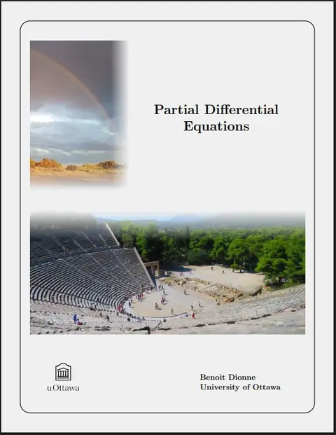
Partial differential equations
Not rated yetRate this bookBenoit Dionne’s Partial Differential Equations develops both explicit solution methods and the analytical framework used to establish existence, uniqueness, and regularity. This guide follows its 13 chapters, from characteristics and classification through wave, Laplace, heat, elliptic, and conservation-law problems.
Free reading is available at the official source. Opens in a new tab.
 Free
About this book
Benoit Dionne’s Partial Differential Equations develops both explicit solution methods and the analytical framework used to establish existence, uniqueness, and regularity. This guide follows its 13 chapters, from characteristics and classification through wave, Laplace, heat, elliptic, and conservation-law problems.
How to study this book
Review multivariable calculus, ordinary differential equations, linear algebra, and basic integration theory before beginning. Keep definitions, hypotheses, and conclusions separate in theorem notes. For every solution, check the equation, domain, boundary or initial conditions, and regularity; a formal expression is not yet a complete verification.
Chapter-wise explanations and study tasks
1. Method of Characteristics
Characteristics convert suitable first-order PDE problems into equations along curves. Initial data determine how these curves are launched, while envelopes and general first-order equations extend the geometry. Examine when the construction is locally valid instead of assuming it always produces a global smooth solution.
Study task: Solve a simple transport initial-value problem by characteristics, sketch the curves, and verify the result directly in the PDE and initial condition.
2. Classification of Partial Differential Equations
The principal part of a second-order equation determines its local classification and guides coordinate changes. Elliptic, hyperbolic, and parabolic equations have different characteristic structures. The chapter extends classification beyond the simplest two-variable constant-coefficient examples.
Study task: Classify three second-order equations using the source’s coefficient convention, then analyse one whose type changes with position.
3. Cauchy Problem
The Cauchy problem asks for a solution compatible with specified data on an initial set. Cauchy–Kovalevski’s theorem gives a result under particular analytic assumptions, while Lewy’s example cautions against broad solvability claims. Record the precise hypotheses rather than remembering only that a theorem guarantees existence.
Study task: State the hypotheses and conclusion of the Cauchy–Kovalevski result in your own words and explain why it does not settle every smooth PDE problem.
4. Review of Functional Analysis
Hilbert spaces, L2 spaces, Fourier series, and operators provide a language for studying solutions beyond pointwise formulas. Distinguish convergence in a norm from pointwise convergence. The Lax–Milgram theorem later becomes a bridge between variational formulations and existence results.
Study task: Work a Fourier-coefficient example and write a separate checklist of the conditions needed to apply Lax–Milgram.
5. Review of Some Special Functions
Frobenius methods and Sturm–Liouville problems connect differential equations with eigenfunctions and orthogonality. Legendre and Bessel functions arise naturally from different coordinate geometries. Learn why the boundary conditions select particular functions instead of treating the chapter as a catalogue of formulas.
Study task: Set up a separated eigenvalue problem in a geometry discussed in the source and identify why its special-function family is appropriate.
6. Distributions and Strong Solutions
Test functions and distributions make differentiation meaningful for objects that are not classically differentiable. Convolution, Fourier transforms, and fundamental solutions provide further analytical tools. Follow the source’s definitions carefully because classical, distributional, and strong-solution terminology carries distinct requirements.
Study task: Compute the distributional derivative of a step function by pairing with a test function, and explain where the resulting point-supported term comes from.
7. Wave Equation in One Dimension
D’Alembert’s method connects initial displacement and velocity with travelling waves. Boundary conditions on half-lines and finite intervals require additional constructions, while forcing and separation of variables provide other solution routes. Verification should include both the initial conditions and any boundary conditions.
Study task: Solve a finite-string example by separation of variables and compare its propagation interpretation with a whole-line d’Alembert solution.
8. Wave Equation in Higher Dimensions
Higher-dimensional wave problems bring energy, uniqueness, spherical geometry, and dimension-dependent propagation into view. Huygens’ principle shows why intuition from one dimension cannot simply be transferred unchanged. Relate the integral representations and separation methods to the domain and data.
Study task: Explain the source’s dimension-dependent propagation discussion with a labelled diagram and outline how an energy argument can establish uniqueness.
9. Laplace Equation
Harmonic functions connect mean-value and maximum principles with boundary-value problems. Green’s functions, Perron’s method, layer potentials, and separation of variables offer different routes to existence or representation. Distinguish Dirichlet data from Neumann data and their associated compatibility and uniqueness issues.
Study task: Solve a simple Dirichlet problem in a rectangle, then explain why a Neumann formulation requires a different compatibility or normalization discussion.
10. Heat Equation
Diffusion evolves initial data through smoothing rather than wave-like transport. Fundamental solutions, forcing, maximum principles, and separated expansions provide complementary viewpoints. Relate time decay and boundary conditions to the behaviour of the modes in a solution.
Study task: Construct a separated solution on a bounded interval, verify its initial and boundary data, and explain the long-time behaviour of its modes.
11. Sobolev Spaces
Weak derivatives and Sobolev norms provide spaces in which PDE solutions can be studied systematically. Density, extension, embeddings, and trace-related ideas explain how approximation and boundary behaviour are handled. Be explicit about which statements concern equivalence classes and which regularity is actually established.
Study task: Test a simple piecewise-defined function for weak differentiability and explain how membership in a Sobolev space differs from classical differentiability.
12. Linear Elliptic Partial Differential Equations
Variational methods formulate elliptic problems through integral identities on function spaces. Coercivity, boundary conditions, and regularity determine what can be concluded about weak solutions. Connect existence and uniqueness arguments to their hypotheses before considering how a weak solution becomes more regular.
Study task: Derive the weak formulation of a homogeneous Dirichlet Poisson problem and identify the function space, bilinear form, and conditions used for existence.
13. Shock Waves
Conservation laws can develop discontinuities even when a classical solution initially exists. Rankine–Hugoniot relations determine admissible jump speeds, while entropy considerations help select physically meaningful weak solutions. The chapter also introduces rarefactions, systems, and approximation approaches.
Study task: For a scalar Riemann problem, compare a shock and a rarefaction construction, compute a jump speed where appropriate, and explain the role of an entropy condition.
Applied assignment
Prepare a comparative PDE notebook containing one transport problem, one wave problem, one heat problem, and one elliptic boundary-value problem. For each give its classification, data, method, verification, and applicable existence or uniqueness statement. Add a short explanation of how a conservation-law shock changes the required solution concept.
Suggested reading plan
Study chapters 1–3 for first-order methods and classification; use 4–6 to establish the functional and distributional tools. Work 7–10 as a sequence of model equations, then 11–12 for Sobolev and variational theory. Study 13 after revisiting characteristics and weak-solution ideas. The longest analytical chapters deserve multiple sessions.
Questions for reflection
- Which hypotheses make a formal PDE calculation legitimate?
- How do boundary conditions change uniqueness?
- Why can a weak solution require an additional admissibility criterion?
Edition and source notes
Based on Benoit Dionne’s 2024 University of Ottawa text, adapted from advanced undergraduate and graduate course notes. The source contains 13 chapters and assumes mathematical prerequisites beyond introductory calculus. This guide supplies original learning prompts, not replacements for the proofs and worked developments.
About access & copyright
This page provides book information and study material. Full-text access is provided by the original publisher or authorised source; a listing does not grant permission to republish the book.
Read our Library Access & Copyright policyExplore the contents
Check the chapters covered in this edition.
Visit the official source
See reading, preview or purchase options.
Save for later
Keep this textbook in your saved collection.
Reader ratings & reviews
Share your thoughts
Your review helps other students choose the right resources.
KEEP LEARNING
Your next great read
alopecia, hair loss, alopecia areata, hair follicle, depression, pathogenesis
 Complex analysis
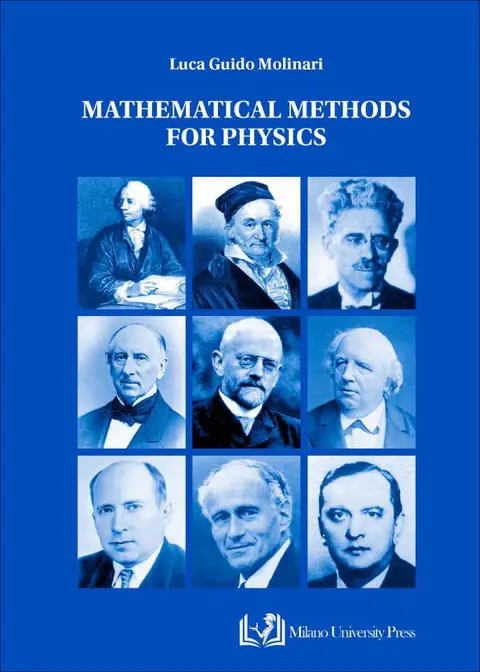
Mathematical Methods for Physics
View Mathematical Methods for Physics — book Biophysics
Principles of Development : An Inquisitive Journey into Embryology
View Principles of Development : An Inquisitive Journey into Embryology — book Communication écrite
Le Littéraire dans le quotidien : Resources for a transdisciplinary approach to reading/writing at the first and second year levels of college French
View Le Littéraire dans le quotidien : Resources for a transdisciplinary approach to reading/writing at the first and second year levels of college French — book Operations Management
View Operations Management — book Communication
Advanced professional communication : A principled approach to workplace writing
View Advanced professional communication : A principled approach to workplace writing — book Early Childhood Education
Children's learning through play
View Children's learning through play — book Budgeting and financial management
Financial Empowerment (2nd Edition)
View Financial Empowerment (2nd Edition) — book Conflict management
Navigating HR : The art of problem-solving and conflict resolution
View Navigating HR : The art of problem-solving and conflict resolution — book Algebra