
 Mathematics
Complex analysisTextbook
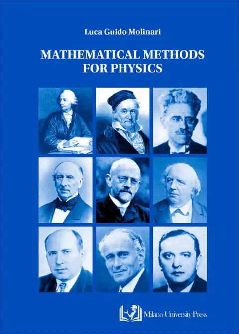
Mathematical Methods for Physics
Not rated yetRate this bookLuca Guido Molinari’s Mathematical Methods for Physics develops complex analysis and functional analysis through proofs, examples, and physical applications. This guide follows the 2026 Milano University Press edition’s twenty-nine chapters, connecting contour methods, function spaces, operators, distributions, and integral transforms.
Free reading is available at the official source. Opens in a new tab.
 Free
About this book
Luca Guido Molinari’s Mathematical Methods for Physics develops complex analysis and functional analysis through proofs, examples, and physical applications. This guide follows the 2026 Milano University Press edition’s twenty-nine chapters, connecting contour methods, function spaces, operators, distributions, and integral transforms.
How to study this book
Review multivariable calculus, linear algebra, and elementary series before starting. For every theorem, record its hypotheses, domain, conclusion, and one example where a missing hypothesis matters. Rework derivations without looking at the next line, draw contours and branch cuts, and distinguish formal manipulation from a justified limit or interchange. The source marks some extension topics with asterisks; use these for a second pass when prerequisites are secure.
Chapter-wise explanations and study tasks
1. Complex Numbers
The historical route through cubic and quartic equations motivates imaginary quantities as tools for solving algebraic problems. Distinguish obtaining a formal expression from checking that its values solve the original equation, especially when roots and branches introduce choices.
Study task: Work through a cubic example that passes through complex intermediate quantities and verify the final candidate roots directly.
2. The Field of Complex Numbers
Conjugation, modulus, argument, exponentials, logarithms, powers, and roots organize arithmetic in the complex field. The argument’s nonuniqueness becomes important when a logarithm or noninteger power is treated as a function.
Study task: Express one number in Cartesian and polar form, enumerate its roots, and explain how choosing an argument interval defines a logarithm branch.
3. The Complex Plane
Lines, circles, stereographic projection, and Möbius maps connect algebraic operations with geometry. Tracking points, exceptional values, and the point at infinity reveals what a transformation actually does rather than only its formula.
Study task: Map a line or circle under inversion and a Möbius transformation, checking the images of selected points and any exceptional point.
4. Sequences and Series
Topology and convergence give precise meaning to limiting processes in the complex plane. Absolute convergence, Cauchy products, and standard series establish operations that need hypotheses rather than unrestricted symbolic rearrangement.
Study task: Compare convergence and absolute convergence for selected series, and state conditions under which a proposed product or rearrangement is justified.
5. Complex Functions
Complex differentiability, Cauchy–Riemann conditions, conformal maps, harmonic functions, and inverse branches connect local analysis with geometry. Satisfying a derivative relation at one point differs from establishing holomorphicity on an open set.
Study task: Test a simple function for complex differentiability and identify a domain on which a chosen logarithm or square-root branch is analytic.
6. Electrostatics
Planar electrostatic examples use harmonic functions and conformal mapping to address conductor boundaries and charge configurations. The transformed function must satisfy the intended boundary conditions; a convenient map alone is not the physical solution.
Study task: Choose a source conductor geometry and trace the mapping, potential boundary values, and interpretation of the resulting field.
7. Complex Integral
Parameterized paths, contour integrals, primitives, the Cauchy transform, and winding index prepare the language for contour theorems. Orientation, path geometry, and the location of singularities affect the value of an integral.
Study task: Evaluate a simple contour integral by parameterization and compute the winding index for the same path around two different points.
8. Cauchy Theorems for Rectangles
The rectangular-domain development establishes a controlled route to Cauchy’s theorem and integral formula. Follow where holomorphicity and the position of the evaluation point enter the argument rather than applying the formula to every closed contour.
Study task: Use the integral formula on a rectangular contour, explicitly checking the integrand’s regularity and the point’s location.
9. Entire Functions
Liouville’s theorem and consequences for polynomials demonstrate how global restrictions constrain holomorphic functions. Boundedness on the entire complex plane is a much stronger condition than boundedness on a selected region.
Study task: Use Liouville’s theorem in a short argument and explain why removing either the global domain or boundedness assumption invalidates the same reasoning.
10. Dixon Theorem and General Cauchy Formula
The contents calls this chapter Dixon Theorem; the chapter develops Cauchy’s theorem and formula for general domains using the index function. Winding conditions account for topology and prevent an integral from ignoring singularities outside the permitted domain.
Study task: Compare a contour in a simply connected domain with one winding around a hole, and identify which index condition permits the general theorem.
11. Power Series
Uniform convergence and power-series structure support differentiation, integration, and generating-function methods. Orthogonal-polynomial examples and the Airy equation show why expansions can be computational tools as well as representations.
Study task: Find a power series’ radius of convergence and use one source generating function to derive its first few polynomial coefficients.
12. Analytic Continuation
Zeros, identity principles, and continuation connect locally defined analytic expressions. The gamma function illustrates extension beyond an initial representation, while singularities and branch structure limit where one formula or branch can apply.
Study task: Continue a simple analytic expression beyond its original series disk and explain why the continued function and the original series have different domains of representation.
13. Laurent Series
Laurent expansions describe holomorphic functions on annuli and connect positive and negative powers with singular behaviour. Bessel, Fourier, and Z-transform examples relate coefficients to other useful representations. The region of expansion is part of the answer.
Study task: Expand one rational function in two different annuli and explain why the resulting coefficient patterns differ.
14. The Residue Theorem
Residues, singularities, contour choices, real integrals, principal values, branch cuts, zeros, poles, and sums form a broad application toolkit. A residue calculation must include orientation, enclosed singularities, and the behaviour of auxiliary contour segments.
Study task: Evaluate a convergent real integral by a suitable contour, justifying the vanishing arc contribution and checking the result by an independent estimate.
15. Elliptic Functions
Elliptic integrals, Jacobi functions, and double periodicity extend the familiar relationship between trigonometric functions and integrals. Follow the chosen definitions and parameters carefully because similar notation can hide different conventions.
Study task: Compare a trigonometric limiting case with an elliptic-function example and explain the role of the parameter and the period structure.
16. Quaternions and Beyond
Quaternion multiplication links algebra with vector operations while abandoning commutativity. The octonion extension introduces another change in algebraic structure. Operations valid for real or complex scalars therefore require reconsideration.
Study task: Multiply two quaternion basis elements in both orders and connect the result with the orientation of a vector cross product.
17. Metric Spaces
Metrics, completeness, maps, and contractions organize convergence independently of coordinates. Completeness concerns whether Cauchy sequences remain inside the space, and it is essential to the fixed-point argument presented here.
Study task: Verify a contraction estimate in a simple complete space and explain why a similar iteration on a noncomplete domain might lose its proposed limit.
18. Banach Spaces
Normed complete spaces, Lp examples, bounded operators, dual spaces, operator algebras, and operator series connect analysis with linear structure. The norm fixes the meaning of convergence and boundedness, so changing it can change the argument.
Study task: Check the norm and completeness questions for a familiar example, then derive a sufficient norm condition for an operator Neumann series to converge.
19. Hilbert Spaces
Inner products add angles, orthogonality, projection, and complete orthonormal systems to the structure of a complete space. L2 examples, orthogonal polynomials, quadrature, and Bargmann space show several realizations of these ideas.
Study task: Project a function onto a finite orthonormal set, calculate the residual norm, and explain the best-approximation property.
20. Trigonometric Series
Fourier expansions, Dirichlet and Fejér constructions, and different convergence modes connect periodic functions with orthogonal representation. Applications include heat flow, vibrating strings, and other physical or mathematical examples. Pointwise agreement and mean-square convergence are distinct claims.
Study task: Compare ordinary partial sums with Fejér sums for a function with a jump and explain what the plots do and do not establish about convergence.
21. Bounded Linear Operators
Functionals, adjoints, projections, unitary and Hilbert–Schmidt operators lead into spectral distinctions. Infinite-dimensional spectra are not exhausted by ordinary eigenvalues, and operator properties depend on the specified space.
Study task: Compare a projection and a unitary operator, then describe a source example distinguishing an eigenvalue from a continuous-spectrum value.
22. Unitary Groups
Stone’s theorem links suitable continuous unitary evolution with a self-adjoint generator. Translations, dilations, rotations, and related representations connect operator families with physical transformations. Track the parameter and convention before differentiating an operator family.
Study task: Examine a translation family, verify its group property, and identify the formal generator while stating the domain questions it raises.
23. Unbounded Linear Operators
Graphs, closedness, adjoints, self-adjointness, and spectral decomposition make operator domains central. Two identical differential expressions can define different operators when their domains or boundary conditions differ.
Study task: Compare the derivative on two specified domains and show how an integration-by-parts boundary term affects the adjoint discussion.
24. Schwartz Space and Fourier Transform
Rapidly decreasing smooth functions provide a setting in which Fourier operations and convolution can be controlled. Seminorms specify the topology, while heat and strip-boundary examples show how transformation simplifies physical equations.
Study task: Verify that a Gaussian is a Schwartz function and use a Fourier-transform calculation to explain a heat-kernel convolution solution.
25. Tempered Distributions
Distributions act on test functions and extend differentiation and transformation beyond ordinary functions. Delta, step, principal-value, response, probability, and generalized-eigenvector examples require attention to the action on tests rather than pointwise pictures.
Study task: Compute the distributional derivative of the step function by its action on a test function and explain why this differs from an ordinary pointwise derivative.
26. Green Functions
Green functions express a system’s response to a point source and connect Helmholtz, oscillator, and wave problems with distributional methods. Boundary or causal conditions select a response; the differential equation alone may not specify it uniquely.
Study task: Compare two possible Green functions for the same differential expression and explain which boundary or causal condition distinguishes them.
27. Fourier Transform II
Fourier theory is extended to L1 and L2 settings, where existence, inversion, and convergence need appropriate interpretations. A transform understood in mean square need not be justified by an absolutely convergent integral at every point.
Study task: Compare an integrable example with a square-integrable example and state the sense in which each Fourier representation is being used.
28. Laplace Transform
The Laplace integral, inversion, convolution, and Mellin-related material connect growth conditions with transform methods. A formula’s convergence region is part of its meaning, and inversion contours must respect analytic structure.
Study task: Compute a simple Laplace transform with its convergence half-plane, then recover it through an inversion or convolution argument with the assumptions stated.
29. Gaussian Integrals and Grassmann Variables
Gaussian integration links quadratic forms with determinants, while anticommuting Grassmann variables obey a different algebra and integration convention. Random-matrix applications illustrate the motivation for these tools. Sign and ordering conventions must remain explicit.
Study task: Compare an ordinary finite-dimensional Gaussian integral with a simple Grassmann integral, identifying how determinant powers and ordering conventions enter.
Applied assignment
Prepare a three-part mathematical-methods portfolio: a residue-based integral, a Fourier or Green-function solution of a physical model, and an operator-domain analysis. For each, state the hypotheses, work through the derivation, check a limiting or solvable case, and explain where a formal manipulation needs justification.
Suggested reading plan
Use eight blocks: chapters 1–5 for complex foundations; 6–10 for physical maps and integration theorems; 11–14 for expansions and residues; 15–16 for extensions; 17–19 for function spaces; 20–23 for series and operators; 24–27 for Fourier methods and distributions; and 28–29 for further transforms and integral techniques. Allow several sessions per block and return to starred topics after the core route is secure.
Questions for reflection
- Which hypothesis allows the theorem to be used here?
- What kind of convergence is required for the operation you performed?
- How do a domain or boundary condition change the mathematical and physical answer?
Edition and source notes
Based on Luca Guido Molinari’s 2026 Milano University Press edition, DOI 10.54103/milanoup.287, whose preface is dated September 1, 2025. Coverage follows all twenty-nine chapters in two parts. Chapter 10’s contents and body use different titles for the Dixon/Cauchy development; both are identified here. The source’s appendix and references remain supporting material in the full text.
About access & copyright
This page provides book information and study material. Full-text access is provided by the original publisher or authorised source; a listing does not grant permission to republish the book.
Read our Library Access & Copyright policyExplore the contents
Check the chapters covered in this edition.
Visit the official source
See reading, preview or purchase options.
Save for later
Keep this textbook in your saved collection.
Reader ratings & reviews
Share your thoughts
Your review helps other students choose the right resources.
KEEP LEARNING
Your next great read
Mathematics Algebra
Fanshawe Pre-Health Sciences Mathematics 2
View Fanshawe Pre-Health Sciences Mathematics 2 — book Algebra
Fanshawe Pre-Health Sciences Mathematics 1
View Fanshawe Pre-Health Sciences Mathematics 1 — book Mathematics
Math 3080 Preparation
View Math 3080 Preparation — book Algebra
Linear Algebra with Applications
View Linear Algebra with Applications — book Business and Economics
Mathematics of Finance
View Mathematics of Finance — book Algebra
The Essence of Mathematics Through Elementary Problems
View The Essence of Mathematics Through Elementary Problems — book complex numbers
Making up Numbers: A History of Invention in Mathematics
View Making up Numbers: A History of Invention in Mathematics — book Business and Management
Inventory Analytics
View Inventory Analytics — book Challenges and roles for textbooks in a pandemic context