
Abstract
Composite filaments are innovative materials designed to elevate artistic 3D printing to new heights. These filaments blend diverse components like wood, metal, or carbon fiber with traditional PLA or ABS plastics, resulting in a versatile medium that enables artists to create visually striking and structurally robust 3D printed artworks. By combining aesthetics and functionality, composite filaments offer a wide range of possibilities for pushing the boundaries of artistic expression in the world of 3D printing. This research work offers a thorough analysis of the material characteristics required to produce high-caliber 3D-printed creative buildings. The tensile strength, modulus, and elongation at break of HDPE/ β -Si3N4 composite filaments were carefully calculated and described. The study investigates the synergistic effects of adding β -Si3N4 nanoparticles to HDPE matrices in an effort to improve the mechanical characteristics of the composite filaments. Furthermore, the Self-Adaptive Tasmanian Devil Optimization Algorithm (SA-TDOA) is utilized to optimize printing parameters, including print speed, and layer height, with the aim of avoiding typical 3D printing issues such as warping, layer adhesion problems, and print discontinuities. The results provide insightful information regarding the viability of applying these composite filaments in artistic 3D printing applications. The optimization procedure has the potential to significantly enhance the accuracy and reliability of 3D printing for artistic endeavors, thereby expanding the possibilities for creative expression in this field. In addition, a new MultiModal Fusion Network is introduced by combing the Convolutional Neural Network, Deep Recurrent Neural Networks with Multi-Layer Perceptron and Deep RNNs with Multi-Layer Perceptron, to enhance the accuracy and reliability of 3D printing for artistic endeavors. The results provide insightful information regarding the viability of applying these composite filaments in artistic 3D printing applications. The optimization procedure has the potential to significantly enhance the accuracy and reliability of 3D printing for artistic endeavors, thereby expanding the possibilities for creative expression in this field. The proposed model has been implemented in MATLAB, for efficient mechanical properties prediction.
Keywords: High-Density Polyethylene, Si3N4 nanoparticles, Tasmanian Devil Optimization, 3D printing
Introduction
Three-dimensional (3D) printing technologies, often known as additive manufacturing (AM), are believed to have revolutionized the manufacturing industry. In recent decades, tremendous advancements in 3D printing and additive manufacturing (AM) have transformed rapid prototyping and the creation of intricate geometries [1]. In certain instances, the accuracy and fine detail offered by 3D printing have made it possible to produce items that would have been inconceivable using conventional manufacturing techniques. Today, industries ranging from aerospace to biomedical engineering recognize its significance [2].
Robocasting is a potential additive manufacturing technique that was first applied two decades ago to create ceramic woodpile scaffold structures [3]. Similar to fused deposition of ceramics, this process involves the extrusion of a filament of paste/ink through a computer-controlled nozzle guided by a CAD model to construct green ceramic pieces layer by layer [4]. A wide variety of materials, including ceramics, metals, polymers, graphene, bioactive substances, and ferroelectric materials, have all been created and printed using this method.
3D printing is a unique manufacturing philosophy that enables the flexible preparation of extremely complex and accurate structures, which can be challenging to produce using traditional fabrication techniques like casting and machining [5]. Ceramics offer numerous advantageous features compared to metals and polymers, such as a high melting point, strong mechanical strength, and exceptional thermal stability [6]. However, these characteristics also pose challenges when creating ceramic components using 3D printing methods [7].
While ceramic 3D printing supports various ceramic materials, the options are still more limited than with conventional ceramic manufacturing techniques [8]. Some specialized or rare ceramic materials may not be readily available for 3D printing, potentially limiting material choices for certain applications [9]. Furthermore, 3D printing in ceramics can be relatively expensive compared to conventional methods [10], with significant upfront costs for materials and equipment. Post-processing steps like sintering may require specialized machinery and consume more energy [11]. The mechanical strength and uniformity of ceramic 3D printed products may not always match those of traditional ceramic production techniques, potentially requiring extensive testing and optimization [12].
One of the main challenges is the excessive shrinkage, porosity, cracking, and deformation caused by the pyrolysis of organic materials used for binding or polymerization in 3D printing [13-14]. Another challenge is the low printing resolution and transparency of translucent ceramics [15].
In this research, we employ the Self Adaptive Tasmanian Devil Optimization Algorithm, a novel hybrid model, to address the limitations of 3D printing in ceramic design. This technique enhances the mechanical strength and widens the temperature range for using the printed composite material. It also improves its resistance to impact damage. The use of polyethylene polymer in 3D printing allows for the manufacturing of components with complex shapes, which is challenging to achieve with current techniques. The inclusion of polyethylene polymer in fiber-reinforced ceramic composites addresses low conductivity issues, increasing the conductivity of the mixture. Additionally, a 3D printing forming tool for ceramic matrix composites has been developed, utilizing liquid resin spray heads and electrostatic spinning technology to achieve photocuring forming of continuous fiber-reinforced composite materials. This approach overcomes challenges associated with 3D printing ceramic structures, such as shape shrinkage and poor densification, by selecting the right material composition and printing techniques.
The study is driven by a comprehensive understanding of how 3D printing using polyethylene composites can enhance the mechanical properties of ceramic structures. It also explores the incorporation of electric field sources into 3D printing processes for in-situ ceramic particle alignment, further improving the composites’ qualities. The objective of this work is to address the drawbacks of 3D printing processes for ceramic structures, including shape shrinkage, mass loss, inadequate densification, and subpar mechanical performance.
The major contribution of this research work is:
To Develop HDPE/β-Si3N4 Composite Filaments: Introduction of a new composite filament blend, merging HDPE and β-Si3N4 nanoparticles, designed to improve 3D printing material performance.
To Quantify Enhanced Mechanical Properties: Thorough analysis and quantification of mechanical properties (tensile strength, modulus, elongation at break) of HDPE/β-Si3N4 composite filaments, showcasing improvements over traditional filaments.
To Investigate Synergistic Effects: In-depth examination of how β-Si3N4 nanoparticles interact with HDPE, elucidating the synergistic effects contributing to the overall mechanical performance of the composite filaments.
To Apply SA-TDOA for Optimization: Innovative use of the Self-Adaptive Tasmanian Devil Optimization Algorithm (SA-TDOA) to optimize critical 3D printing parameters such as print speed, and layer height, addressing common printing issues.
To introduce a new MultiModal Fusion Network, seamlessly combines the power of Convolutional Neural Networks (CNN), Deep Recurrent Neural Networks (RNNs) with Multi-Layer Perceptron (MLP), and Deep RNNs with Multi-Layer Perceptron, representing a holistic approach to enhance the accuracy and reliability of the 3D printing process.
The remaining sections of this research project are structured as follows: Section II covers the literature related to the subject, Section III discusses the proposed technique, Section IV presents the test results, and Section V concludes the research.
Literature Review
Sajadi et al. 2021 [16] introduced a straightforward method to externalize the soft phase by applying a conformal polymer coating on designed ceramic structures, resulting in enhanced damage tolerance. They utilized a silica-filled preceramic polymer to print architectural structures, which were subsequently pyrolyzed to stabilize the ceramic scaffolds. These structures were then dip-coated conformally with a thin, flexible epoxy polymer. This surface modification technique significantly increased compressive strength, toughness, and delayed damage propagation. It offers the potential to create intricate and damage-tolerant ceramic pieces.
Drawbacks: The intrinsic brittleness of ceramics poses a significant challenge in 3D printing, as it can lead to frequent breakage and catastrophic failure. There is a need to enhance the damage resistance of 3D-printed ceramic structures to make them more robust and reliable.
Lube et al. 2023 [17] outlined the challenges and possibilities for improving the mechanical properties of printed ceramics, focusing on brittle failure within the context of linear elastic fracture mechanics. They discussed various printing-related challenges, including surface quality, geometry control, printing directions, and the need for testing procedures for 3D printed items. The study also explored bio-inspired material design concepts to enhance the mechanical resistance of 3D-printed ceramics based on layer-by-layer stereolithographic capabilities, achieving high strength and fracture resistance by customizing layer architecture and microstructure.
Drawbacks: 3D printing of ceramics faces challenges related to their brittle nature and the potential introduction of flaws during the printing process. These issues hinder the mechanical performance of 3D-printed ceramics, and there is a need to explore solutions to improve their mechanical characteristics.
Park et al. 2022 [18] provided a brief history of AM technologies and discussed filling materials for structural and functional applications, including 3D printing polymers. They covered the physical and chemical properties of polymers and filling materials, along with the fundamentals of additive manufacturing processes. The study explored new uses for 3D printed polymers and composites, such as applications in biology, electrical energy storage, electronics, and robotics. It also highlighted potential challenges and difficulties in AM of polymer composites, offering insights into future research directions.
Drawbacks: Despite the rapid advancement of polymer and composite 3D printing, several challenges persist, such as material selection, process optimization, and addressing specific application needs. To further advance the technology, it is essential to understand these challenges and explore potential solutions.
Jiang et al. 2023 [19] summarized the performance of 3D printed sensing materials and devices, along with state-of-the-art 3D printing methods for manufacturing sensors. The development of MultiMate rial printing and 4D printing technologies was discussed, aiding the creation of multifunctional structures. The study encompassed various sensor types, including piezoelectric sensors, medical sensors, and optical sensors, comparing the performance of 3D-printed sensors to conventionally manufactured ones. The section also provided insights into the future development of 3D printed sensors.
Drawbacks: As 3D printing gains popularity for creating sensors due to its precision and versatility, there is a need to assess the effectiveness of 3D printed sensing materials and devices. Additionally, advancements in 3D printing techniques for sensor manufacturing need to be explored to meet the growing demand for innovative sensors.
Pollak et al. 2021 [20] investigated the possibility of creating 3D printing filaments from granular PLA material Ingeo 2003D by mixing it with fiber from selected PLA material and glass powder filler. They used the FilaFab PRO EX350 machine for fiber extrusion, aiming to develop novel materials and components made from ecologically benign materials, gradually replacing currently utilized materials.
Drawbacks: The study addresses the need to develop new 3D printing materials that offer improved strength and resilience compared to conventional PLA. Additionally, there is a need to explore ecologically friendly materials for 3D printing to promote sustainability in the field.
Johnson et al. 2021 [21] outlined the manufacturing process for fully 3D-printed ceramic core structures for portable solar desalination units, addressing water scarcity from an energy and sustainability perspective. The study used a 3D printing technology called robocasting to create a ceramic structure with an integrated solar absorber, thermal insulator, and water transporter. The technique involved modified graphene on silica and porous silica structure, offering flexibility in modifying structural designs to achieve uniform water delivery and thermal insulation.
Drawbacks: With increasing water scarcity in various regions, there is a demand for portable solar desalination units. The challenge lies in creating efficient and entirely 3D-printed ceramic core structures that can quickly produce clean drinking water, addressing both energy and sustainability concerns.
Zhang et al. 2021 [22] investigated the fundamental photocuring units using cordierite ceramic slurries loaded with different average particle sizes. They used digital light processing (DLP) based on photocuring, altering exposure times to achieve a range of ultraviolet light-energy dosages. The study examined the morphologies, structures, and dimensional changes of printed units before and after processing stages, gaining insights into ceramic slurries’ and printed units’ behaviors and performances in photocuring-based DLP 3D printing.
Drawbacks: Understanding the behavior of cordierite ceramic slurries during the 3D printing and sintering process is essential for improving the quality and reliability of ceramic components produced using photocuring-based DLP 3D printing. This research addresses this need.
Lozynskyy et al. 2021 [23] focused on producing high-density polyethylene or polypropylene using -Si3N4 powder to create ceramic-reinforced polymer materials. They conducted research on integrating silicon nitride ceramic particles with polymers to create polymer-ceramic filaments. The study produced high-quality polypropylene-ceramic filaments and polyethylene-ceramic filaments using an extrusion process. Mechanical and tribological characteristics of the materials were investigated, and various polymer-ceramic pieces were printed to evaluate filament quality.
Drawbacks: To create robust 3D printing materials, there is a need to investigate the integration of ceramic reinforcements, such as -Si3N4 powder, with polymers like high-density polyethylene or polypropylene. The challenge lies in optimizing the composite materials to enhance their mechanical properties for various applications.
Sun et al. 2022 [24] examined computational tools for ceramic product design and a three-dimensional strategy for design management. They investigated the use of 3D printing technology in the ceramics industry, highlighting the role of machines in ceramic 3D printing processes and the properties of 3D printed ceramic Modeling. The study designed and created various ceramic shapes using ceramic 3D printing technology, aligning with the principles of aesthetics and Modeling design.
Drawbacks: While Sun set al.’s study focused on computational tools for ceramic product design and 3D printing technology in the ceramics industry, it did not extensively address specific challenges or limitations faced by this technology. The study may benefit from a more comprehensive analysis of obstacles encountered in ceramic 3D printing processes and their potential solutions. Additionally, a deeper exploration of the practical applications and industrial scalability of ceramic 3D printing could provide valuable insights into its real-world implementation.
Zhou et al. 2020 [25] explored 3D printing techniques for creating polymer-derived ceramics (PDC). They discussed the advantages and disadvantages of preceramic polymers compared to ceramic powders, providing insights into material selection, structure design, and the creation of dependable custom 3D printed PDC components. The study emphasized the potential benefits of preceramic polymers and their role in designing functional 3D printed PDC devices.
Drawbacks: the study did not delve deeply into the potential drawbacks or challenges associated with the use of preceramic polymers in 3D printing. A more balanced assessment of both the benefits and limitations of this approach could offer a more comprehensive understanding of its feasibility and applicability in various contexts. Additionally, the study could have explored practical case studies or applications of 3D printed PDC components to demonstrate their real-world utility and potential drawbacks in specific industries or scenarios.
Methods
Laminated Object Manufacturing (LOM) is a process for 3D printing that deposits material sheets layer-by-layer, which are coated with adhesive to build complex three-dimensional objects. The foremost phase of the LOM process encompasses the development of a 3D model of the object that is required to be printed using various software tools, particularly computer-aided design (CAD) software, which cannot be executed. The pattern is subsequently sliced into narrow sections, where the thickness of each section is determined by the materials utilized and the preferred printing precision. Subsequently, the LOM printer is loaded with the material sheets, and the first layer is deposited on the build platform before applying a thin layer of adhesive with a roller. The opening layer is contoured through a laser or blade, and the resulting layers are placed atop one another until the object is fully constructed. It might be important to undertake post-processing activities like removing excess material, sanding, or painting for the printed object.
The adaptable 3D printing method known as LOM can be used to create prototypes, models, and completed parts. It is a technique that is reasonably quick and inexpensive, and it works with a variety of materials. LOM is less accurate than certain other 3D printing methods, making it difficult to create elaborate objects with fine details.
Methodology
A high-density polyethylene (HDPE) matrix combined with -Si3N4 powder is used in the procedure to create polymer-ceramic composite filaments for 3D printing. The composite filaments were developed to bring together the enhanced characteristics of ceramics and the mechanical capabilities of polymers. Before being crushed in alcohol to a particular surface area of 3.8 cm2/g, -Si3N4 powder is first created by self-propagating high-temperature synthesis. The particle size distribution is investigated with the aid of computer analysis and optical microscopy.
To guarantee homogeneous dispersion, the HDPE polymer and -Si3N4 powder are physically combined in a ceramic crucible at temperatures between 130°C and 180°C. In order to create filaments with a diameter of 1.75 0.05 mm, the resulting composite mixture is extruded using a Well zoom desktop extruder at temperatures as high as 300°C and an extrusion speed of 30 cm/min. The complicated structures are then produced using the composite filaments in Ultimaker Plus 3D printers. The 3D printed objects are tested for their mechanical and thermal qualities after the 3D printing parameters are changed as necessary.
Experimental Procedure
Factual Gaining and Grounding: Polypropylene homopolymer of grade Alkom PP 620/10 and high-density polyethylene (HDPE) of grade 2210J were used to construct the polymer matrix. -Si3N4 powder obtained via self-propagating high-temperature synthesis had a specific surface area of 3.81 cm2/g after being ground in alcohol for 36 hours. The particle size distribution was determined using an optical microscope and image processing.
Compound Development: In a ceramic crucible, the polymer matrix and -Si3N4 powder were mechanically combined. The composite was homogeneous since the mixing took place between 130°C and 180°C. Care was taken during the mixing process to prevent the introduction of air bubbles.
Fiber Extrusion: The combined composite material was processed using the Well zoom desktop extruder. The extruder’s operating temperature was increased to a maximum of 300 °C to aid in the extrusion procedure. The composite material was fed into the extruder’s feed hopper and extruded at a controlled rate of no more than 30 cm/min. A spool was filled with extruded filaments that were 1.75 0.05 mm in diameter.
3D Printing Practice: On the Ultimaker + 3D printer, items were created using the composite filaments. The composite filament was put into the 3D printer’s filament holder. Variables like extrusion temperature, print speed, and layer height were adjusted as necessary for the optimum printing outcomes. After selecting a certain 3D model, the printing process was initiated.
Post-Printing Steps: The finished 3D-printed objects were left to cool to room temperature before any post-processing was carried out. This can require removing support structures or carrying out other finishing tasks specified by the design.
Assessment and Classification: The appropriate testing techniques were used to assess the printed products’ mechanical and thermal properties. We compared the qualities of composite polymer-ceramic goods and pure polymer materials.
Data Investigation and Explanation: Evaluation data were studied to determine the efficacy and calibre of the polymer-ceramic composite products produced. The results were interpreted in light of the purposes for adding ceramics to the polymer matrix and any potential advantages.
Reproducibility and quality assurance: The entire experimental procedure was carried out under controlled conditions to ensure repeatability. The approach, parameter settings, and observations were well documented in order to allow for the method’s replication to be trusted. Figure 1 shown in below.
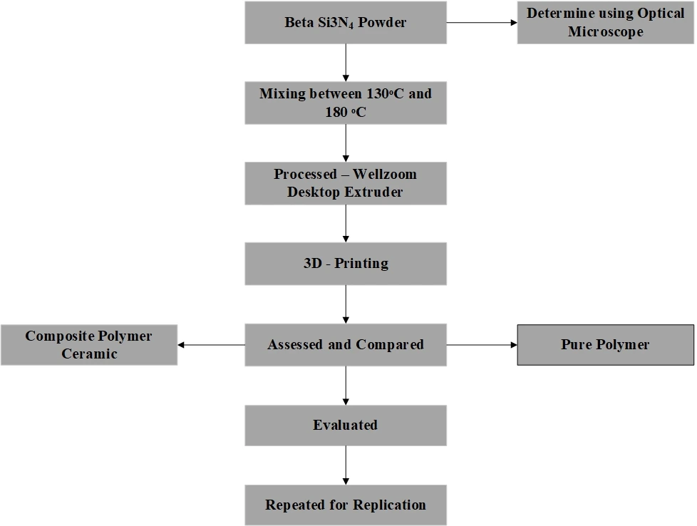
Figure 1: Experimental procedure Polymer Matrix
Self Adaptive Tasmanian Devil Optimization Algorithm
SA-TDOA is an advanced optimization algorithm inspired by the hunting behavior of Tasmanian devils, a carnivorous marsupial native to Australia. This algorithm mimics the devils’ hunting strategies, which involve adaptively adjusting their tactics based on the success of previous hunts. In 3D printing, the quality and success of a print job depend on several key parameters, including nozzle temperature, print speed, and layer height. These parameters affect factors such as layer adhesion, material flow, and overall print accuracy. Therefore, the
Inspiration and Behaviour of the Tasmanian Devil
The Tasmanian devil is a carnivorous and marsupial wild animal belonging to the family Dasyuridae that lives in the island state of Tasmania. Tasmanian devils are opportunistic animals, and although they are able to hunt prey, they feed on carrion if present. Tasmanian devil has two strategies for feeding. In the first strategy, if Tasmanian devil finds a carrion, it feeds on it. In the second strategy, it hunts and feeds on prey by attacking it. The modeling of this Tasmanian devil feeding mechanism is used in the SA-TDOA design.
Mathematical Modelling
In this subsection, the process and how to simulate the natural behaviour of Tasmanian demons during feeding is described to design an optimizer.
The optimization process is how to achieve the optimal solution for an optimization issue. The analogy of this process in the life and behaviours of the Tasmanian devil is like access to food. In fact, just as in the optimization process, the goal is to find the optimal solution, in the Tasmanian devil’s nutritional process, the goal is to find the food source. Two important principles in the optimization process are exploration in the comprehensive search the problem-solving space and exploitation in approaching the optimal solution. The Tasmanian devil’s search behaviour in finding food sources in different spaces, in fact, indicates the exploration index in the optimization process in order to identify the optimal area of search space. On the other hand, the chasing process between the Tasmanian devil and the prey that occurs in a limited area is similar to the exploitation index in the local search with the aim of converging to the optimal solution. This means that mathematical modeling of Tasmanian devil strategies to reach the food source is prone to designing an optimizer to achieve optimal solutions to optimization problems. SA-TDOA utilizes an objective function that quantifies the quality of the ongoing print. The algorithm’s goal is to maximize this objective function, which translates to achieving the best possible print quality.
Initialization
The proposed SA-TDOA is a population-based stochastic algorithm whose searcher agents are Tasmanian devils. The initial population of these agents is generated randomly based on the constraints of the problem. Population members of SA-TDOA, who are searchers of problem-solving space, suggest candidate values for problem variables based on their position in the search space. So mathematically, each member of a population is a vector with the number of elements equal to the number of problem variables. As a result, the set of SA-TDOA members can be modelled using a matrix in (1).
X= [[X1] ; [⋮] ; [[X2] ; [⋮] ; [X3]]]N×m=⌊[x1,1 , ⋯ , x1,j , ⋯ , x1,m] ; [⋮ , ⋱ , ⋮ , ⋰ , ⋮] ; [xi,1 , ⋯ , xi,j , ⋯ , xi,m] ; [⋮ , ⋰ , ⋮ , ⋱ , ⋮] ; [xN,1 , ⋯ , xN,j , ⋯ , xN,m]⌋N×m (1)
where X is the population of Tasmanian devils, Xi is the i th candidate solution while xi,j is its candidate value for the j th variable, N is the number of searching Tasmanian devils, and m is the number of variables of given problems.
The objective function of problem can be computed by placing each of the candidate solutions in the values of the variables of the objective function. As a result, the values obtained for the objective function are modelled using a vector in (2).
F= [[F1] ; [⋮] ; [Fi] ; [⋮] ; [FN]] =[[F(X1)] ; [⋮] ; [F(Xi)] ; [⋮] ; [F(XN)]]N×1 (2)
where F is the vector of values of the objective function and Fi is the value of the objective function obtained by the i th candidate solution. The analysis of the values obtained for the objective function shows the quality of the candidate solutions. The candidate solution that leads to the calculation of the best value for the objective function is considered the best member of the population. The best member of the population is updated based on new values in each iteration.
The population updating process in SA-TDOA is modelled on two Tasmanian devil feeding strategies. It is possible for any Tasmanian devil to eat carrion or feed on prey hunting. In SA-TDOA, it is assumed that the probability of choosing any of these strategies is equal to 50%. According to this concept, in each iteration of the SA-TDOA, each Tasmanian devil is updated based on only one of these two strategies.
Strategy 1: Brownian Motion based Feeding by Eating Carrion (Exploration Phase) (proposed)
Tasmanian devils exhibit a feeding strategy where they scavenge for carrion in their habitat, especially when other predators have hunted large prey but can’t consume it entirely. This behavior draws parallels to how the SA-TDOA algorithm explores different areas of the problem-solving space to find the optimal solution. Random selection of one of these situations is simulated in (3) so that the k' th population member is selected as the target carrion for the i' th Tasmanian devil. Therefore, k must be chosen randomly from 1 to N while the opposite is i.
Ci=Xk, i=1,2,…,N,kϵ {1,2,…, N|k ≠i} (3)
where Ci is the selected carrion by i th Tasmanian devil. Once the carrion is selected, the Tasmanian devil explores the problem space by moving towards or away from it, depending on whether the carrion’s objective function value is better or worse, respectively.
In SA-TDOA design, each Tasmanian devil represents a potential solution within the problem space. The algorithm simulates the Tasmanian devil’s behavior by selecting one of its fellow population members as if it were carrion, essentially picking a “target” solution to guide its motion. This motion is influenced by Brownian motion in SA-TDOA. Mathematically, this motion, or change in position, influenced by Brownian motion, is simulated as:
Calculate the new position for the Tasmanian devil based on the selected carrion and Brownian motion:
If FCi <Fi (if carrion is better), the Tasmanian devil moves closer to the carrion with Brownian motion. If not, it moves away from the carrion with Brownian motion. This Tasmanian devil’s motion strategy, now incorporating Brownian motion, is defined as:
xi,jnew, S1= {xi,j+r. (ci,j-I. xi,j)+ Brownian_Motion, FCi <Fi; ; xi,j+r. (xi,j– ci,j)+ Brownian_Motion, otherwise, (4)
Finally, after calculating the new position with Brownian motion, it’s accepted if the objective function value is better in this new position; otherwise, the Tasmanian devil remains in its previous position. Brownian_Motion represents the influence of Brownian motion on the motion. This strategy incorporates Brownian motion to emulate the Tasmanian devil’s scavenging behavior while exploring the problem-solving space in a more dynamic and diverse manner. It enhances the SA-TDOA algorithm’s ability to find optimal solutions, particularly in complex optimization scenarios.
Xi= {Xinew, S1, Finew, S1<Fi; ; Xi, otherwise, (5)
Here, Xinew, S1 is the new status of the i th Tasmanian devil based on the first strategy, xi,jnew, S1 is its value for the j th variable, Finew, S1 is its objective function value, FCi is its objective function value of selected carrion, r is a random number in interval [0,1] , and I is a random number which can be 1 or 2.
Strategy 2: Carrion Feeding and Gaussian-Based Random Walk (Exploitation Phase) (proposed):
The Tasmanian Devil’s second feeding strategy is to hunt and eat prey. Tasmanian devil behavior during the attack has two stages. In the first stage, by scanning the area, it selects the prey and attacks it. Then, in the second stage, after approaching the prey, it chases it to stop it and start eating. The modeling of the first stage is similar to the modeling of the first strategy, i.e., the selection of the carcass. Therefore, the first stage of prey selection and attack is modeled using equations (6) to (8). In the second strategy, when updating the i' th Tasmanian devil, the position of other population members is assumed as preys’ location. The k' th population member is randomly selected as prey, while k is a natural random number between 1 to N and opposite i. The prey selection process is simulated in (6).
Prey Selection with Gaussian-Based Random Walk:
Instead of Levy flight, you can incorporate a Gaussian distribution-based random walk into the prey selection process. This random walk generates small steps in a controlled manner, allowing the Tasmanian devils to explore the solution space more effectively while reducing the risk of large, uncontrolled leaps.
Pi= Xk+ Gaussian_Random_Walk, i=1,2,…,N,k ϵ {1,2,…, N ; k≠i}, (6)
Here, Pi is the selected prey by the i th Tasmanian devil. In addition, Gaussian_Random_Walk represents the random walk vector generated from a Gaussian distribution and applied to the prey’s location.
Gaussian-Based Random Walk Simulated Prey Selection:
After determining the prey position, a new position is calculated for the Tasmanian devil. In calculating this new position, if the objective function value of the selected prey is better, the Tasmanian devil moves towards it, otherwise it moves away from that position. Modelling of this process is presented in (7). The new position calculated for the Tasmanian devil replaces the previous position if it improves the value of the target function. This step of the second strategy is modelled in (8).
xi,jnew, S2= {xi,j+r. (pi,j-I. xi,j), FPi <Fi; ; xi,j+r. (xi,j– pi,j), otherwise, (7)
Position Update with Gaussian-Based Random Walk: This updated position is accepted by the Tasmanian devil if it improves the value of the target function compared to its previous position. This position update process is simulated for the Tasmanian devil in equation (8).
Xi= {Xinew, S2, Finew, S2<Fi; ; Xi, otherwise, (8)
Here, Xinew, S2 is the new status of i' th Tasmanian based on the second strategy, xi,jnew, S2 is its value for the j th variable, Finew, S2 is its objective function value, and FPi is its objective function value of selected prey.
The main difference between this strategy and the first strategy is the second stage and the simulation of prey chasing. The chase of prey in the vicinity of the attack site is similar to the local search of the search space. This Tasmanian devil behaviour actually demonstrates the SA-TDOA’s ability to exploit to converge to better candidate solutions. In order to simulate this chase process, the Tasmanian devil follows the prey in the neighbourhood of the attacked place. The prey chase stage is modelled by the Tasmanian devil using (9) to (11). At this stage, the Tasmanian devil position is considered the centre of a neighbourhood where the prey chasing process takes place. The radius of this neighbourhood indicates the range that the Tasmanian devil follows the prey, which can be calculated using (9). Thus, a new position based on the chasing process in this neighbourhood can be calculated for the Tasmanian devil, which is mathematically simulated in (10). The new calculated position is acceptable to the Tasmanian devil if it provides a better value for the objective function than its previous position. This position update process is simulated for the Tasmanian devil in (11).
R=0.01 (1- (t)/(T)) (9)
xi,jnew= xi,j+(2r-1). R. xi,j (10)
Xi= {Xinew, Finew<Fi, ; Xi, otherwise, (11)
where R is the neighbourhood radius of the point of attacked location, t is the iteration counter, T is the maximum number of iterations, Xinew is the new status of the i th Tasmanian devil in neighbourhoods of Xi, xi,jnew is its value for the jth variable, and F new i is its objective function value.
Repetitions process, flowchart, and pseudo-code of SA-TDOA
When the update of all SA-TDOA members is completed, the first iteration of the algorithm ends. New values are calculated for the position of Tasmanian devils and the objective function. After this, the algorithm enters the next iteration and the SA-TDOA population update process continues until the end of the algorithm iterations according to equations (3) to (11). SA-TDOA updates and stores the best candidate solution during these iterations. After the algorithm is fully implemented, SA-TDOA introduces the best candidate solution as the solution to the problem. The various steps of SA-TDOA are presented in flowchart format in Figure 2 and its pseudocode in Algorithm 1.
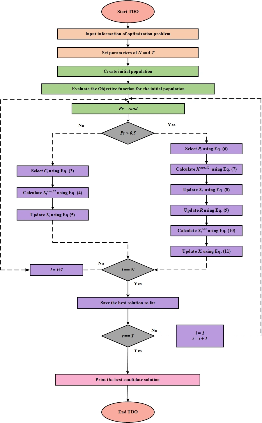
Figure 2: Flow chart SA-TDOA
Algorithm 1: Pseudo-Code of Proposed SA-TDOA
Start
1. Input the optimization problem information.
2. Set the number of iterations (T) and the number of
members of the population (N).
3. Initialization of the position of Tasmanian devils and
evaluation of the objective function.
4. For t D 1: T
6. For i D 1: N
8. If Probability < 0.5, Probability D rand
9.Strategy 1: Feeding by eating carrion (exploration phase)
10. Select carrion for the ith Tasmanian devil using
Eq. (3).
11.Calculate new status of Tasmanian devil using
Eq. (4).
12.Update the ith Tasmanian devil using (5).
13.else
14.Strategy 2: Feeding by eating prey (exploitation phase)
15.Stage 1: Prey selection and attacking
16.Select prey for the ith Tasmanian devil using (6).
17. Calculate new status of Tasmanian devil using
Eq. (7).
18. Update the ith Tasmanian devil using (8).
19. Stage 2: Prey chasing
20. Update neighbourhood radius using (9).
21. Calculate new status of the ith Tasmanian devil in
neighbourhood of Xi using (10).
22. Update the ith Tasmanian devil using (11).
23.end if
24.end for i D 1: N
25.Save the best proposed solution so far.
26. end for t D 1: T
27.Output: The best solution obtained by SA-TDOA for given
optimization problem.
Terminate
Multimodal Fusion Network
In this research, we present a pioneering contribution to the field of 3D printing for artistic endeavors by introducing a novel “MultiModal Fusion Network.” This MultiModal Fusion Network is shown in Fig.3. This advanced network architecture seamlessly combines the power of Convolutional Neural Networks (CNN), Deep Recurrent Neural Networks (RNNs) with Multi-Layer Perceptron (MLP), and Deep RNNs with Multi-Layer Perceptron, representing a holistic approach to enhance the accuracy and reliability of the 3D printing process. Convolutional Neural Network (CNN): The CNN component processes image data, capturing visual features and patterns from images of artistic designs and objects. It excels at extracting spatial information and identifying visual elements critical for 3D printing. Deep Recurrent Neural Networks (Deep RNNs) with Multi-Layer Perceptron (MLP): This part of the network handles sequential and textual data, allowing the model to understand and interpret the artistic intent, design specifications, and any relevant textual information. Deep RNNs, combined with MLP, can capture intricate sequential dependencies and nonlinear patterns in text data. By integrating these diverse data modalities and leveraging sophisticated neural network components, the MultiModal Fusion Network enhances the accuracy and reliability of 3D printing specifically for artistic endeavors. It ensures that artistic designs are faithfully translated into 3D printed artworks with precision and quality. Figure 3 shown in below.
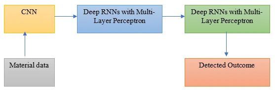
Figure 3: MultiModal Fusion Network
Convolutional Neural Network
Convolutional neural networks (CNNs) – or convnets, for short – have in recent years achieved results which were previously considered to be purely within the human realm. In this chapter we introduce CNNs, and for this we first consider regular neural networks, and how these methods are trained. After introducing the convolution, we introduce CNNs. They are very similar to the regular neural networks as they are also made up of neurons with learnable weights. But, in contrast to MLPs, CNNs make the explicit assumption that inputs have specific structure like images. This allows encoding this property into the architecture by sharing the weights for each location in the image and having neurons respond only locally. CNN is done using weight optimized via Self Adaptive Tasmanian Devil Optimization Algorithm.
Intuitively, this means that when training such a CNN, the network will learn filters that capture some kind of visual information such as an edge, orientation, and eventually, in a higher layer of the network, entire patterns. In each such convolution layer, we have an entire set of such filters, each of which will produce a separate activation map. These activation maps are stacked to obtain the output map or activation volume of this layer.
Mathematically, the convolution (x * w)(a) of functions x and w is defined in all dimensions as
(x * w)(a)= ∫(x(t)w(a-t)da) (12)
where a is in Rn for any n≥ 1, and the integral is replaced by its higher-dimensional variant. To understand the idea behind convolutions, it is interesting to pick the Gaussian function w(a) = exp(-x2) as an example. If we were taking a photo with a camera and shaking the camera a bit, the blurry picture would be the real picture x convolved with a Gaussian function w.
In the terminology of convolutional neural networks, x is called the input, w is called the filter or kernel, and the output is often referred to as activation, or feature map. Note that we modeled the input and kernel in (12) as a continuous function. Due to the discrete nature of image sensors, this will not be the case in practice and it is more realistic to assume that parameter t is discrete. If we assume that this is the case, then we can define the discrete convolution.
(x * w)(a)= ∑a(x(t)w(t – a)) (13)
where a runs over all values in the space, and can be in any dimension. In deep learning, usually x is a multidimensional array of data and the kernel w involves learnable parameters and usually has finite support, that is, there are only finitely many values a for which w(a) is nonzero. This means that we can implement (13) as a finite summation. The definition of (13) is independent of dimension, but in medical imaging we will mainly be working with 2- or 3-dimensional convolutions:
(I * K)(i,j)= ∑m(∑n(I(m, n)K(i – m,j – n),)) (14)
or
(I * K)(i,j, k)= ∑m(∑n(∑l(I(m, n, l)K(i – m,j – n, k – l)))) (15)
The convolutions (14) and (15) are commutative, which means that I *K = K * I, so that we can also write (14) as:
(I * K)(i,j) = ∑m(∑n(I(i – m,j – n)K(m, n))) (16)
As K has finite support, this a priori infinite sum becomes finite. Some neural network libraries also implement an operation called the cross-correlation, but from a deep learning perspective these operations are equivalent, as one weight set can be directly translated into the other.
Deep RNNs with Multilayer Perceptron
Deep architectures of neural networks can represent a function exponentially more efficient than shallow architectures. While recurrent networks are inherently deep in time given each hidden state is a function of all previous hidden states, it has been shown that the internal computation is in fact quite shallow. In, it is argued that adding one or more nonlinear layers in the transition stages of a RNN can improve overall performance by better disentangling the underlying variations the original input. The deep structures in RNNs with perceptron layers can fall under three categories: input to hidden, hidden to hidden, and hidden to output.
Deep input to hidden: One of the basic ideas is to bring the multi-layer perceptron (MLP) structure into the transition and output stages, called deep transition RNNs and deep output RNNs, respectively. To do so, two operators can be introduced. The first is a plus ⊕ operator, which receives two vectors, the input vector x and hidden state h, and returns a summary as
h ' = x ⊕ h (17)
The other operator is a predictor denoted as ⊳, which is equivalent and predicts the output of a given summary h as
y = ⊳h (18)
Higher level representation of input data means easier representation of relationships between temporal structures of data. This technique has achieved better results than feeding the network with original data in speech recognition and word embedding applications.
Deep hidden to hidden and output: The most focus for deep RNNs is in the hidden layers. In this level, the procedure of data abstraction and/or hidden state construction from previous data abstractions and new inputs is highly nonlinear. An MLP can model this non-linear function, which helps a RNN to quickly adapt to fast changing input modes while still having a good memory of past events. A RNN can have both an MLP in transition and an MLP before the output layer. A deep hidden to output function can disentangle the factors of variations in the hidden state and facilitate prediction of the target. This function allows a more compact hidden state of the network, which may result in a more informative historical summary of the previous inputs.
Recurrent Convolutional Neural Networks
The rise in popularity of RNNs can be attributed to its ability to model sequential data. Previous models examined have augmented the underlying structure of a simple RNN to improve its performance on learning the contextual dependencies of single dimension sequences. However, there exists several problems, which require understanding of contextual dependencies over multiple dimensions. The most popular network architectures use convolutional neural networks (CNNs) to tackle these problems. CNNs are very popular models for machine vision applications. CNNs may consist of multiple convolutional layers, optionally with pooling layers in between, followed by fully connected perceptron layers. Typical CNNs learn through the use of convolutional layers to extract features using shared weights in each layer. The feature pooling layer (i.e., subsampling) generalizes the network by reducing the resolution of the dimensionality of intermediate representations (i.e., feature maps) as well as the sensitivity of the output to shifts and distortions. The extracted features, at the very last convolutional layer, are fed to fully connected perceptron model for dimensionality reduction of features and classification. Incorporation of recurrent connections into each convolutional layer can shape a recurrent convolutional neural network (RCNN). The activation of units in RCNN evolve over time, as they are dependent on the neighbouring unit. This approach can integrate the context information, important for object recognition tasks. This approach increases the depth of model, while the number of parameters is constant by weight sharing between layers. Using recurrent connections from the output into the input of the hidden layer allows the network to model label dependencies and smooth its own outputs based on its previous outputs. This RCNN approach allows a large input context to be fed to the network while limiting the capacity of the model. This system can model complex spatial dependencies with low inference cost. As the context size increases with the built-in recurrence, the system identifies and corrects its own errors. Quad-directional 2-dimensional RNNs can enhance CNNs to model long range spatial dependencies. This method efficiently embeds the global spatial context into the compact local representation.
Results and Discussion
Study limitations. The numerical results and equations are reproduced as reported. The MSE and RMSE values do not satisfy the stated relationship for a common evaluation set, and the MARE equation repeats the numerator in its denominator. Model labels in the discussion differ from those in Table 1. Sample counts, filler loadings and the prediction evaluation split are insufficiently specified. These limitations prevent independent verification of the claimed performance and mechanical improvements.
Performance Metrics
The mechanical strength prediction has been done using MATLAB tool. Evaluation is done in terms of error measures such as Mean Absolute Error, Mean Squared Error, Root Mean Square Error, Correlation, Mean Absolute Relative Error. Moreover, the proposed model has been validated over the existing models like MDRNN (Multi-Dimensional Recurrent Neural Network), BRNN (Bidirectional Recurrent Neural Network), DRNN (Deep Recurrent Neural Network), MLP (Multi-Layer Perceptron), and CNN (Convolutional Neural Network), respectively.
Mean Absolute Error Definition
The term “mean absolute error” (MAE) refers to the average of mistakes between paired observations that reflect the same phenomena. Examples of Y against X include contrasts between expected and observed data, subsequent time and starting time, and one measuring technique and another measurement technique. The MAE is determined by dividing the total absolute errors by the sample size.
MAE=(∑i=1n(|yi-xi|))/(n) (19)
Mean Squared Error Definition
The average of the squares of the errors, or the average squared difference between the estimated values and the actual value, is measured by the mean squared error (MSE) or mean squared deviation (MSD) of an estimator (of a process for estimating an unobserved variable). The predicted value of the squared error loss corresponds to the risk function known as MSE.
MSE=(1)/(n)∑i=1n((y1-yî)2) (20) 4.1.3 Root Mean Square Error
In order to evaluate how different disease symptoms affect the effectiveness of the treatments used at various disease severity levels, RMSE is used in this study.
RMSE=√((1)/(N)(Av-Pv)2) (21)
Correlation Definition
Any statistical association between two random variables or bivariate data, whether causal or not, is referred to as correlation or dependency. Although “correlation” can mean any kind of link in the widest sense, in statistics it often refers to how linearly connected two variables are to one another.
Mean Absolute Relative Error Definition
The average percent difference between the actual and anticipated values is calculated using MARE. It does so by expressing the mistake as a % of the actual numbers, which can be helpful when attempting to gauge the relative accuracy of forecasts.
MARE=(1)/(N)∑i=1N(|(yt-ft)/(yt-ft)|) (22)
Table 1: Performance of error metrices
Proposed | MDRNN | BRNN | DRNN | MLP | CNN | |
MAE | 7.462 | 8.384 | 7.844 | 8.109 | 10.095 | 9.074 |
MSE | 89.752 | 105.8 | 99.548 | 111.356 | 145.321 | 133.037 |
RMSE | 10.407 | 11.449 | 10.851 | 10.983 | 12.064 | 12.16 |
Correlation | 0.94 | 0.89 | 0.85 | 0.92 | 0.82 | 0.88 |
MARE | 0.22 | 0.252 | 0.808 | 0.941 | 1.104 | 1.029 |
Mean Absolute Error Results
Table 1 shows that effectiveness of different neural network architectures was evaluated using the Mean Absolute Error (MAE) performance metric in a proposed comparison study of MDRNN (Multi-Dimensional Recurrent Neural Network), BRNN (Bidirectional Recurrent Neural Network), DRNN (Deep Recurrent Neural Network), MLP (Multi-Layer Perceptron), and CNN (Convolutional Neural Network). With an MAE of 7.462, the MDRNN outperformed the other models in terms of predicted accuracy. The MAE values of 8.384 and 7.844 for the BRNN and DRNN, respectively, showed how competitive they were in their performance. The MLP and CNN, on the other hand, had higher MAE values of 8.109 and 10.095, respectively, indicating they would be less appropriate for the particular task or dataset in question. These results show that MDRNNs have the capacity to make precise predictions, which has ramifications for their usage in different fields that call for sequential data processing. It may be possible to optimize the performance of these models with more research and parameter modification. The performance analysed graph is mentioned below Figure 4.
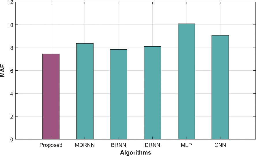
Figure 4: Performance analysed in terms of MAE
Mean Squared Error Results
Table shows that mean squared error (MSE) performance, the proposed Multiple-Input, Multiple-Output (MDRNN) model appears to perform better than other architectures in the context of machine learning and neural networks, such as Bidirectional Recurrent Neural Networks (BRNN), Deep Recurrent Neural Networks (DRNN), Multi-Layer Perceptrons (MLP), and Convolutional Neural Networks (CNN). The MDRNN specifically has the lowest MSE of 89.752, indicating that it is the best model for reducing prediction errors among the choices taken into consideration. The MDRNN is a promising option for jobs requiring precise sequence modeling and prediction because of its capacity to capture complex relationships in the data through its numerous input and output connections, which is the cause of its better performance. The performance analysed graph is mentioned below Figure 5.
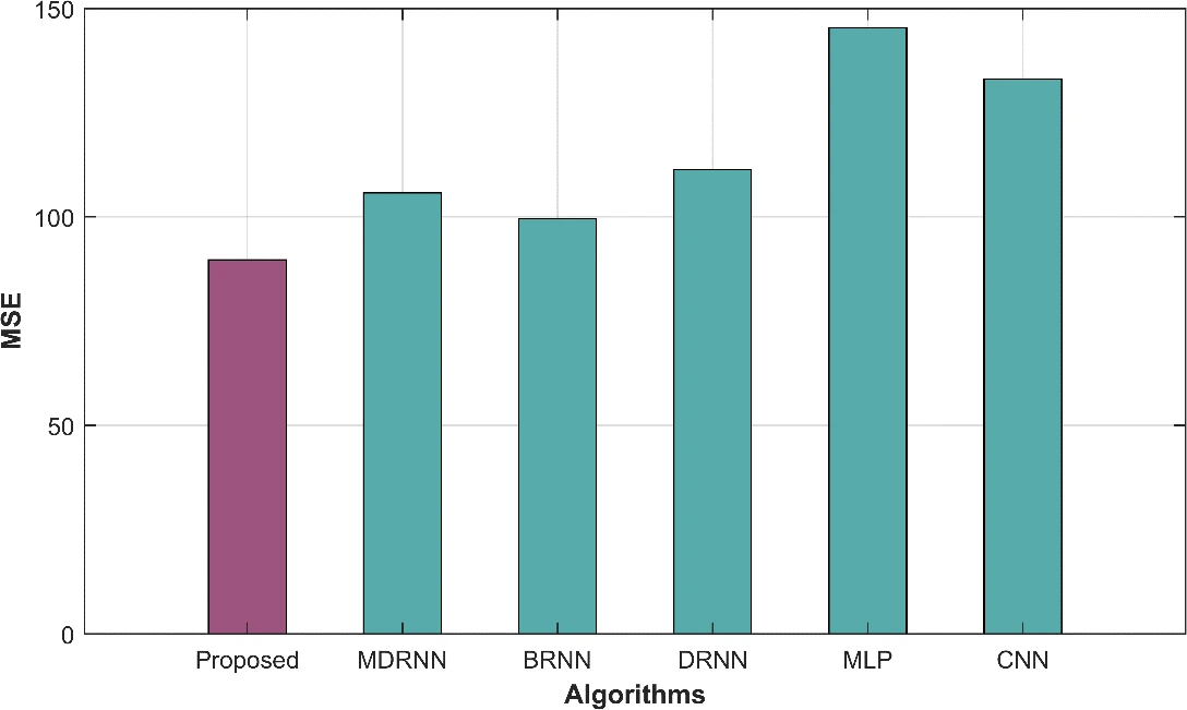
Figure 5: Performance analysed in terms of MAE
Root Mean Square Error Results
Table shows that different neural network designs, including MDRNN, BRNN, DRNN, MLP, and CNN, were evaluated in the context of a proposed machine learning model assessment based on how well they performed in terms of RMSE (Root Mean Square Error). In comparison to the other designs, the MDRNN displayed the lowest RMSE of these models, at 10.407, demonstrating higher predictive accuracy. With RMSE values of 11.449 and 10.851, respectively, the BRNN and DRNN came in second and displayed competitive performance. The RMSE values for the MLP and CNN models, however, were higher, at 10.983 and 12.064, respectively, indicating less effective prediction skills. The MDRNN is shown to be a potential choice for the job in these results because to its superior performance in reducing prediction errors. For possible applications in the real world, more research and confirmation of the MDRNN’s capabilities may be necessary. The performance analysed graph is mentioned below Figure 6.
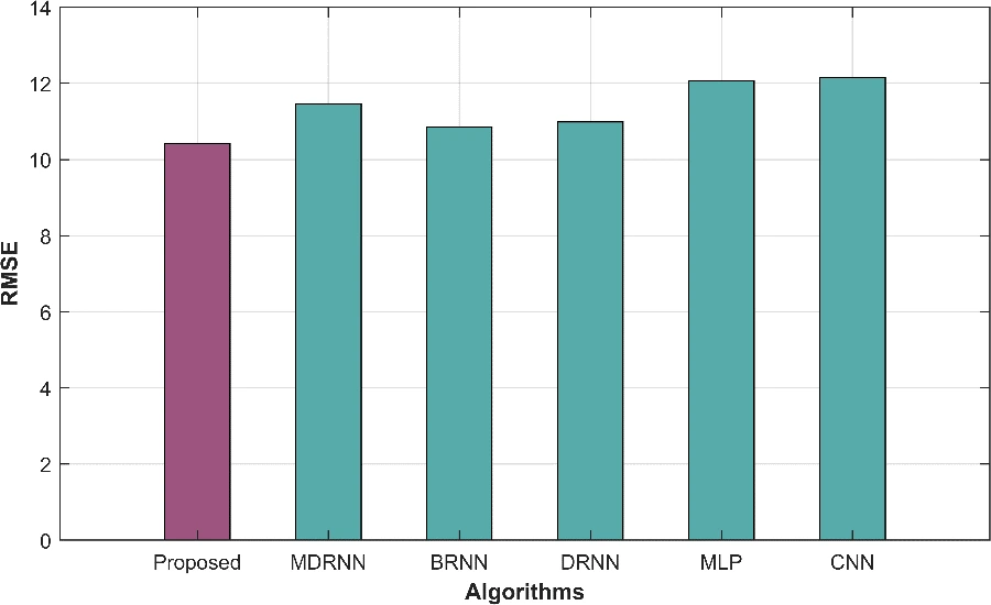
Figure 6: Performance analysed in terms of RMSE
Correlation Results
Table shows that the proposed MDRNN (Multidimensional Recurrent Neural Network) demonstrates impressive performance with a correlation coefficient of 0.94, indicating its superior ability to capture complex relationships within the data. In comparison, the BRNN (Bidirectional Recurrent Neural Network) and DRNN (Deep Recurrent Neural Network) also perform well but exhibit slightly lower correlations of 0.89 and 0.85, respectively, suggesting that they may not capture the temporal dependencies in the data as effectively as the MDRNN. Meanwhile, the MLP (Multilayer Perceptron) and CNN (Convolutional Neural Network) models show moderate correlations of 0.92 and 0.82, respectively, indicating their reasonable performance but trailing behind the MDRNN. The performance analysed graph is mentioned below Figure 7.
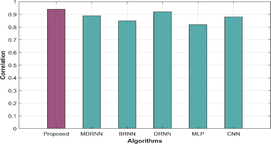
Figure 7: Performance analysed in terms of Correlation
Mean Absolute Relative Error Results
Several other neural network architectures, such as BRNN (Bidirectional Recurrent Neural Network), DRNN (Deep Recurrent Neural Network), MLP (Multilayer Perceptron), and CNN (Convolutional Neural Network), are inferior to the proposed MDRNN (Multidimensional Recurrent Neural Network) based on their Mean Absolute Relative Errors (MARE) for a particular task. In comparison to the BRNN (0.252), DRNN (0.808), MLP (0.941), and CNN (1.104), the MDRNN exhibits greater prediction accuracy with a substantially lower MARE of 0.22. This shows that the MDRNN is especially well-suited for capturing intricate patterns and relationships in the data, giving it a potential option for applications where precise forecasting or modeling of sequential data is crucial. For applications demanding exact predictions, more research and assessment of the MDRNN’s capabilities may be necessary. Performance analysed in terms of MARE is shown diagrammatically in Figure 8.
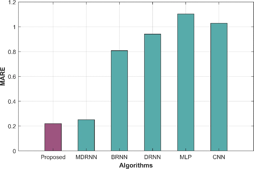
Figure 8: Performance analysed in terms of MARE
Conclusion
This research delves into the utilization of composite filaments, which combine materials like wood, metal, or carbon fiber with plastics in 3D printing, aimed at elevating the quality of 3D-printed buildings. Through a comprehensive analysis of material characteristics, including tensile strength, modulus, and elongation at break, the study investigates the synergistic effects of introducing β-Si3N4 nanoparticles to enhance mechanical properties. Leveraging the Self-Adaptive Tasmanian Devil Optimization Algorithm, the research optimizes crucial 3D printing parameters such as print speed and layer height to mitigate issues like warping and layer adhesion. Furthermore, the introduction of a novel MultiModal Fusion Network, which integrates Convolutional Neural Networks (CNNs), Deep Recurrent Neural Networks (DRNNs), and Multi-Layer Perceptrons (MLPs), seeks to enhance accuracy and reliability in 3D printing. The results reveal the Multi-Deep Recurrent Neural Network (MDRNN) as the top performer, with an impressive Mean Absolute Error (MAE) of 7.462, demonstrating its potential for precise predictions. This breakthrough not only expands creative possibilities in 3D printing but also suggests applications in various fields requiring sequential data processing, promising significant advancements in both artistic and practical domains. The study encourages further research and parameter refinement to maximize the potential of these innovative models.
References
Ian Gibson, I.G., 2015. Additive manufacturing technologies 3D printing, rapid prototyping, and direct digital manufacturing.
Ortiz-Acosta, D. and Moore, T., 2019. Functional 3D printed polymeric materials. Functional materials, 9, pp.1-5.
Malik, U., Selvakannan, P.R., Mazur, M., Li, Y. and Bhargava, S.K., 2022. Robocasting—Printing Ceramics into Functional Materials. In Additive Manufacturing for Chemical Sciences and Engineering (pp. 109-136). Singapore: Springer Nature Singapore.
Bai, J., Sun, J. and Binner, J., 2022. Additive Manufacturing of Ceramics: Materials, Characterization and Applications. In Additive Manufacturing: Materials, Functionalities and Applications (pp. 245-331). Cham: Springer International Publishing.
Shaukat, U., Rossegger, E. and Schlögl, S., 2022. A review of multi-material 3D printing of functional materials via vat photopolymerization. Polymers, 14(12), p.2449.
Alizadeh-Osgouei, M., Li, Y. and Wen, C., 2019. A comprehensive review of biodegradable synthetic polymer-ceramic composites and their manufacture for biomedical applications. Bioactive materials, 4, pp.22-36.
Zhang, D., Jonhson, W., Herng, T.S., Ang, Y.Q., Yang, L., Tan, S.C., Peng, E., He, H. and Ding, J., 2020. A 3D-printing method of fabrication for metals, ceramics, and multi-materials using a universal self-curable technique for robocasting. Materials Horizons, 7(4), pp.1083-1090.
Ly, M., Spinelli, S., Hays, S. and Zhu, D., 2022. 3D printing of ceramic biomaterials. Engineered Regeneration, 3(1), pp.41-52.
Egorov, V., Gulzar, U., Zhang, Y., Breen, S. and O’Dwyer, C., 2020. Evolution of 3D printing methods and materials for electrochemical energy storage. Advanced Materials, 32(29), p.2000556.
Varghese, G., Moral, M., Castro-García, M., López-López, J.J., Marín-Rueda, J.R., Yagüe-Alcaraz, V., Hernández-Afonso, L., Ruiz-Morales, J.C. and Canales-Vázquez, J., 2018. Fabrication and characterisation of ceramics via low-cost DLP 3D printing. Boletín de la Sociedad Española de Cerámica y Vidrio, 57(1), pp.9-18.
Sanicola, H.W., Stewart, C.E., Mueller, M., Ahmadi, F., Wang, D., Powell, S.K., Sarkar, K., Cutbush, K., Woodruff, M.A. and Brafman, D.A., 2020. Guidelines for establishing a 3-D printing biofabrication laboratory. Biotechnology Advances, 45, p.107652.
Dizon, J.R.C., Espera Jr, A.H., Chen, Q. and Advincula, R.C., 2018. Mechanical characterization of 3D-printed polymers. Additive manufacturing, 20, pp.44-67.
Naveed, N., 2021. Investigate the effects of process parameters on material properties and microstructural changes of 3D-printed specimens using fused deposition modelling (FDM). Materials Technology, 36(5), pp.317-330.
Xu, X., Zhang, J., Jiang, P., Liu, D., Jia, X., Wang, X. and Zhou, F., 2022. Direct ink writing of aluminum-phosphate-bonded Al2O3 ceramic with ultra-low dimensional shrinkage. Ceramics International, 48(1), pp.864-871.
Wang, H., Liu, L.Y., Ye, P., Huang, Z., Ng, A.Y.R., Du, Z., Dong, Z., Tang, D. and Gan, C.L., 2021. 3D printing of transparent spinel ceramics with transmittance approaching the theoretical limit. Advanced Materials, 33(15), p.2007072.
Sajadi, S.M., Vásárhelyi, L., Mousavi, R., Rahmati, A.H., Kónya, Z., Kukovecz, Á., Arif, T., Filleter, T., Vajtai, R., Boul, P. and Pang, Z., 2021. Damage-tolerant 3D-printed ceramics via conformal coating. Science Advances, 7(28), p. eabc5028.
Lube, T., Staudacher, M., Hofer, A.K., Schlacher, J. and Bermejo, R., 2023. Stereolithographic 3D printing of ceramics: challenges and opportunities for structural integrity. Advanced engineering materials, 25(7), p.2200520.
Park, S., Shou, W., Makatura, L., Matusik, W. and Fu, K.K., 2022. 3D printing of polymer composites: Materials, processes, and applications. Matter, 5(1), pp.43-76.
Jiang, Y., Islam, M.N., He, R., Huang, X., Cao, P.F., Advincula, R.C., Dahotre, N., Dong, P., Wu, H.F. and Choi, W., 2023. Recent advances in 3D printed sensors: materials, design, and manufacturing. Advanced Materials Technologies, 8(2), p.2200492.
Pollak, M.A.R.T.I.N., Kocisko, M., Basistova, A.N.N.A. and Hlavata, S., 2021. Production of fiber as an input material for the 3D printing process. MM Sci. J, 6, pp.4414-4419.
Jonhson, W., Xu, X., Zhang, D., Chua, W.T., Tan, Y.H., Liu, X., Guan, C., Tan, X.H., Li, Y., Herng, T.S. and Goh, J.C.H., 2021. Fabrication of 3D-printed ceramic structures for portable solar desalination devices. ACS Applied Materials & Interfaces, 13(19), pp.23220-23229.
Zhang, C., Luo, Z., Liu, C., Zhu, J., Cao, J., Yuan, J., Wang, P., Liu, C., Lao, C. and Chen, Z., 2021. Dimensional retention of photocured ceramic units during 3D printing and sintering processes. Ceramics International, 47(8), pp.11097-11108.
Zgalat-Lozynskyy, O.B., Matviichuk, O.O., Tolochyn, O.I., Ievdokymova, O.V., Zgalat-Lozynska, N.O. and Zakiev, V.I., 2021. Polymer materials reinforced with silicon nitride particles for 3D printing. Powder Metallurgy and Metal Ceramics, 59, pp.515-527.
Sun, X., Liu, X., Yang, X. and Song, B., 2022. Computer-aided three-dimensional ceramic product design. Computer-Aided Design and Applications, 19(S3), pp.97-107.
Zhou, S., Mei, H., Chang, P., Lu, M. and Cheng, L., 2020. Molecule editable 3D printed polymer-derived ceramics. Coordination Chemistry Reviews, 422, p.213486.
Cite This Work
To export a reference to this article please select a referencing stye below:

Academic Master Education Team is a group of academic editors and subject specialists responsible for producing structured, research-backed essays across multiple disciplines. Each article is developed following Academic Master’s Editorial Policy and supported by credible academic references. The team ensures clarity, citation accuracy, and adherence to ethical academic writing standards
Content reviewed under Academic Master Editorial Policy.





