
Abstract
This paper investigates an MRI-based research model for multiclass Alzheimer’s disease (AD) classification, combining image security with deep learning. The ADMRI workflow first uses a stream cipher (SC) to secure medical brain images; the encrypted image is then decrypted using the corresponding key. Stream ciphers are considered for their execution speed and comparatively low complexity. Images from the Alzheimer’s Disease Neuroimaging Initiative (ADNI) database are processed using a convolutional neural network (CNN). Transfer learning uses a pretrained AlexNet model for medical-image classification. Jellyfish optimisation (JFO) tunes the learning rate and model parameters, with the rectified linear unit (ReLU) serving as an activation function. The fine-tuned Optimal Deep AlexNet (ODAN) model is reported to achieve 97% accuracy for multiclass AD-stage classification. The results are compared with methods described in the literature. The model is an experimental image-classification approach rather than a clinically validated diagnostic system.
Keywords: Alzheimer’s Disease (AD), classification, Multistage classifier, Convolution network, deep learning, medical images, and optimization
Introduction
Magnetic resonance imaging (MRI) is widely used in neuroradiology to detect brain lesions including stroke, vascular disease, and tumour tissue [1]. Thus, accurate diagnosis of AD and its early stage using a non-invasive and widely available technology is critically important [2]. The main bottleneck to early AD detection is the need for more of the public’s general knowledge about this disease. As a result, cognitive decline and related behaviours are often mistaken for phenomena associated with the normal ageing process and other psychiatric disorders [3]. Early AD diagnosis is chiefly associated with Mild Cognitive Impairment (MCI) detection [4], an early AD stage. While the MCI’s memory complaints as well as deficits do not have a notable impact on the patients’ everyday activities, it has been reported that MCI does have a high risk of progression to AD or other dementia forms [5]. Commonly stream encryption algorithms are used for image encryption [6]. Stream ciphers are built using a pseudorandom key sequence, and then this sequence is combined with the original text through exclusive-or operator. Generally, stream encryption systems have suitable performance when speed and error probability of data transmission are high [7]. In low-level security encryption, the encrypted image has degraded visual quality compared to that of the original one, but the content of the image is still visible and understandable to the viewers [8].
Stream ciphers retain an operating state for subsequent encryption, whereas block ciphers process data in blocks [9]. Conventional machine-learning techniques can be limited in their ability to process raw data directly [10]. A deep convolutional neural network (CNN) uses successive transformations and receptive fields to classify image information. Its features are learned from training images [11] through a general-purpose learning procedure rather than being designed manually [12]. Medical images are complex: characteristics associated with AD, such as hippocampal shrinkage, may also be observed in normally ageing brains [13].
We expect the model to distinguish AD images from those in the other groups. Classification of MCI is also relevant because it can precede AD, although progression is not inevitable [15]. Earlier identification may support further clinical assessment and management [15]. The contributions of this ADMRI study are outlined below.
We propose an optimised convolutional model that combines stream-cipher image security with AlexNet-based ADMRI classification.
The approach uses AlexNet within a Siamese architecture and a feature-vector function for multiclass AD classification. A cipher component is included to support medical-image security and privacy.
A jellyfish search optimisation (JSO) strategy tunes AlexNet layers, learning rates and weights. Four conventional algorithmic approaches are used to evaluate the proposed structure’s classification performance.
A stacking method is proposed that uses ODAN to combine predictions of base classifiers and cope with their dependencies.
A comparative study evaluates the methods using the ADNI dataset and confusion-matrix measures.
The remainder of the paper is organised as follows. Section 2 reviews ADMRI classification research. Section 3 explains the proposed Optimal Deep AlexNet model. Section 4 discusses the experimental results. Section 5 presents the conclusion and future research directions.
Literature Review
Chen & Xia et al in 2021 [16] had proposed the Iterative Sparse and Deep Learning (ISDL) technique to diagnose AD as well as MCI. Initially, a Deep Feature Extraction (DFE) mechanism was designed to identify the local-to-global structural information of sixty-two cortical regions. Afterwards, a sparse regression unit was designed to detect the critical cortical regions, and then to incorporate it into the DFE mechanism for exclusion of the inappropriate cortical regions from the diagnostic procedure. Results of the experimentations had proved that ISDL model was able to offer a highly advanced solution to the AD-CN classification as well as the MCI-to-AD prediction.
Singh and Janghel [17] proposed a hybrid ant-colony optimisation (ACO) and feed-forward CNN strategy for AD classification in 2022. Bio-inspired algorithms identify CNN hyperparameters and recommend a configuration for training. The validation procedure assesses whether images are classified as normal or AD. The reported performance comprises 98.67% accuracy, 97.63% sensitivity and 99.02% specificity.
In 2022 Priyanka Nedunchellian & Ganesan [18] investigated the onset in brain dementia by studying the left and right ventricle variations. The Dual Deep Learning Techniques (DDLT) with optimizations were used in the proposed technique. Multilevel threshold based GWO was used for segmenting ventricle region. The symmetry is checked using the palindrome detection method. AlexNet and ResNet classified the DDLT features. Experimental results concluded that the left ventricle variation can be used as a distinct indicator for differentiating various classes of dementia.
Shaji et al. [19] reported in 2022 that the Extreme Learning Machine (ELM) and its variants could classify AD using morphometric features. With a sigmoid activation function, ELM classifiers achieved accuracy above 90% for both studied regions. Among the variants, SaDE-ELM attained maximum sensitivities of 97% and 94% using lateral ventricle (LV) and corpus callosum (CC) features, respectively, with the lowest number of hidden neurons. LV features showed greater discriminative ability than CC features.
Garg et al. [20] reviewed structural MRI-based studies of AD detection and prediction of MCI-to-AD conversion. Their discussion associates memory loss and declining cognitive ability with brain changes caused by neuronal loss. The reviewed detection framework comprises feature extraction, feature selection and classification. Comparisons suggest that wavelet-transform-based feature extraction offers promising results for AD classification.
In 2023, de Mendonça et al. [21] proposed MR-image classification using graph kernels constructed from structural MRI texture features. Their method first segments brain images into multiple regions with FreeSurfer, then removes graph edges using a threshold-based approach and constructs graph-kernel matrices. Support vector machines (SVMs) perform classification with two graph kernels. The reported AUC values were 0.92 for CN–AD, 0.81 for CN–MCI and 0.78 for MCI–AD classification.
Helaly et al. [22] used CNNs to classify four stages of the AD spectrum in 2021. They also performed separate binary classifications for pairs of stages and discussed stage-dependent patient support. Nine metrics were used to evaluate and compare the approaches. The reported CNN architectures had relatively simple structures intended to reduce computational complexity, memory requirements, overfitting and execution time.
Proposed Methodology
Brain-image processing is an active area of research into brain disorders. The proposed system combines preprocessing, image security, feature extraction and classification. For protected transmission, images are separated into blocks and processed using a key matrix within the stream-cipher method. The encryption and decryption sides must use compatible keys so that the image can be recovered correctly. Figure 1 presents the proposed architecture.
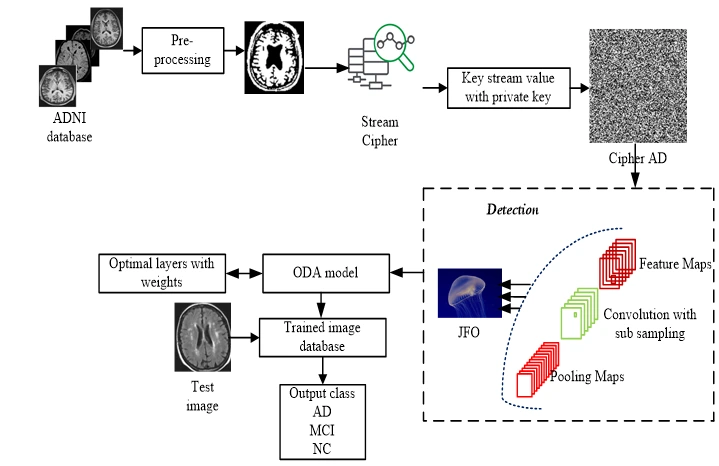
Figure 1: Methodology for AD detection
The proposed deep-learning approach uses an optimised AlexNet convolutional model to classify features extracted from secured brain images. MRI images are obtained from the Alzheimer’s Disease Neuroimaging Initiative (ADNI). The trained classifier assigns each test image to AD, MCI or normal control (NC). The following subsections describe the workflow.
MRI Pre- processing
MRI preprocessing uses an adaptive-histogram approach to improve visual contrast, brightness and image consistency. Grayscale images are used for brain-image segmentation. Any colour MRI images are therefore converted to grayscale before processing [23].
Securing MRI Image: Cipher model
The medical image is represented as text using ASCII characters. A mutated character-code table then encodes those characters to form the plain-image representation. The proposed stream-cipher method encodes both the keystream keys and the characters representing the binary image. A one-time pad offers its stated secrecy properties when the key meets the necessary randomness and usage conditions.
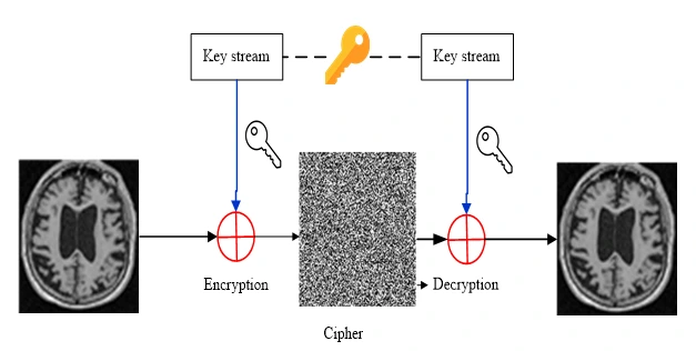
Figure 2: Stream cipher Model
The encrypted binary image is obtained by applying an exclusive-OR (XOR) operation to the key values and the plain-image values [24]. Figure 2 illustrates the stream-cipher model. The encryption and decryption operations are expressed below.
Enc: (1)
Dec:  (2)
 (3)
In Equation (3), the 128-bit key 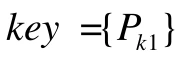 is used with a 32-bit string. The symbol
 denotes the bitwise exclusive-OR operation in the cipher-image calculation.
Encryption and Decryption process
The values are calculated using the preceding equations when the plain-image representation is longer than the keystream in Equation (4).
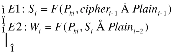 (4)
The receiver uses the encrypted binary image and the encryption-key values to recover an estimate of the plain image.
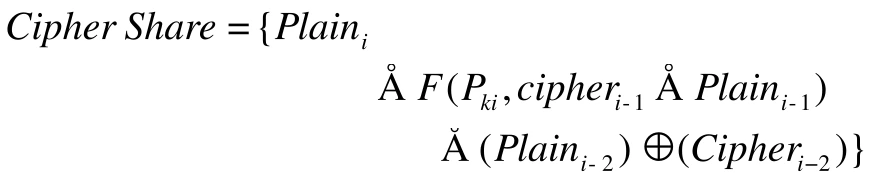 (5)
Stream key process
Inputs: Plain MRI Image
Generate a keystream for the plain image.
Generate the binary-sequence blocks using the linear procedure.
Iterate from i = 1 to N.
Produce the cipher image using the keystream and the private key.
The decoding procedure recovers the encoded image using the common encryption-key set, as expressed below.
 (6)
At the receiver, the encrypted binary image is processed using the keystream estimates and initial values. The receiver must therefore know the key values used during encryption.
Alzheimer’s detection Deep Convolutional AlexNet: ADMRI
The CNN workflow comprises medical-image preparation, model training and testing. The training model learns associations in the secured images. Larger image inputs can increase computational cost, so a feature extractor combines convolutional and pooling layers to transform low-level information into higher-level features. Figure 3 shows the general AlexNet structure.
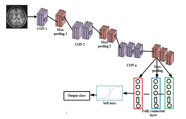
Figure 3: Sample AlexNet structure
Automatic feature extraction reduces manual effort, while weight sharing reduces the number of parameters. The proposed technique combines the deep AlexNet network (DAN) with JSO to select CNN parameters. The training structure shown in Figure 3 uses ReLU activation and batch normalisation to support generalisation.
ReLU Function
ReLU is a half-wave rectifier function used to accelerate training. AlexNet uses ReLU in place of traditional sigmoid and tanh activation functions [25]. Its nonsaturating form can help address vanishing-gradient behaviour and support deeper-network training. Equation (7) defines the activation function.
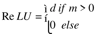 (7)
Activation functions transform the outputs of neural-network layers. Batch normalisation and CNN optimisation are used to support training and medical-image processing [25]. In the described model, the third convolutional layer uses ReLU, 64 filters and a 3 × 3 kernel.
Feature extractor in CNN
Feature extraction represents secured MRI data through characteristics useful for classification while reducing the amount of information that must be processed. The number of convolution kernels corresponds to the number of output feature maps. Multiple kernels learn different features; increasing their number can improve the model’s representational capacity within the limits of the architecture and training data.
CNN-layer Optimization model
Feature extraction aims to identify useful characteristics that distinguish one sample from another. These features support classification of brain MR images into AD, MCI or NC. Jellyfish optimisation (JFO) tunes the layers of the classification system, referred to here as ODAN-ADMRI. The following subsection describes the optimisation procedure.
Jellyfish Optimization (JFO)
JFO models transitions between jellyfish movement with ocean currents and movement within a swarm. Its population, movement and search mechanisms are illustrated in Figure 4. The proposed optimisation mechanism follows three rules [26].
Jellyfish follow ocean currents or move within a swarm. A time-control mechanism regulates transitions between these movement types.
Jellyfish search for food and are attracted towards locations with greater food availability.
Food availability corresponds to the objective-function value at a candidate location. In this application, candidate solutions represent pretrained AlexNet parameters. The weights determine the convolutional responses and pooling-related feature representations of ADMRI data.
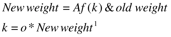 (8)
The AlexNet configuration is tuned to improve learning in the image-processing workflow. Optimising the learning rate and network layers aims to maximise classification performance.
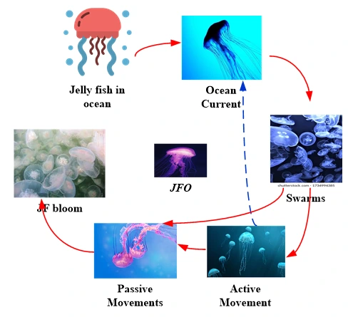
Figure 4: JFO mechanism
(i) Objective function
The fitness of each candidate solution is evaluated using classification accuracy as the principal criterion. At each iteration, the fitness function is calculated as follows.
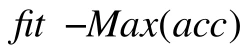 (9)
Equation (9) uses correctly classified and incorrectly classified cases, with WC and WN denoting wrongly classified positive and negative cases in the source notation.
(ii) New updating procedure of DAN
Ocean Current
The ocean-current direction  guides the jellyfish towards food-rich areas and is formulated below.
 (10)
Here,  denotes the current best jellyfish position. Equation (11) gives the updated position;
 represents the position of the
 jellyfish at time
 .
 (11)
Jellyfish Swarm
Jellyfish exhibit different forms of movement within a swarm. Type I movement updates the position of a jellyfish locally, as expressed below.
 (12)
Here,  and
 denote the upper and lower bounds of the search space, respectively. The movement coefficient
 controls the distance travelled around a jellyfish position. The model then updates movement direction and position.
 (13)
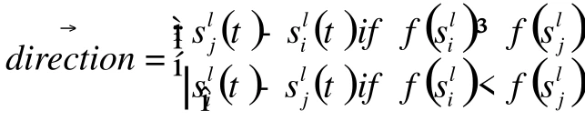 (14)
In Equations (13) and (14), another jellyfish  is selected at random. A vector from the jellyfish of interest
 to the selected jellyfish determines movement direction. The relative food availability at the two positions determines whether movement is towards or away from the selected location.
(iii) Time Control Mechanism for Switching Movements of Jellyfish
Changes in ocean conditions motivate transitions between movement types. The time-control mechanism  is defined in Equation (15). Above the threshold
 , the jellyfish follows the ocean current; below the threshold , it moves within the swarm. The control value varies between zero and one.
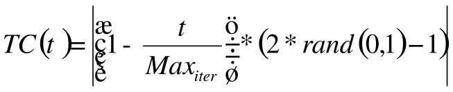 (15)
Here, represents the  iteration, and
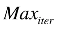 denotes the maximum number of iterations. The objective function selects the best result, and the cycle repeats until the maximum iteration count is reached.
Optimal Deep AlexNet approach: ODAN
The CNN model contains four convolutional blocks and two fully connected layers. Each convolutional block comprises convolution, pooling, batch normalisation and Leaky ReLU. The final fully connected layers support classification, as illustrated in Figure 5.
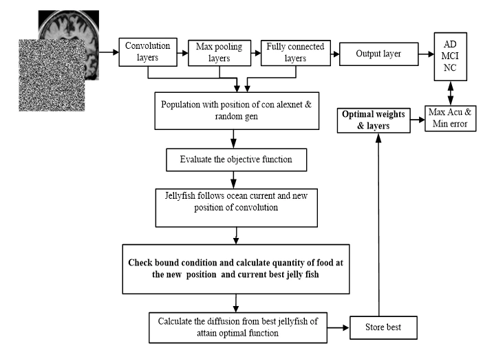 Figure 5: Convolution AlexNet – JFO model
Network training begins with randomly initialised weights. Softmax activation converts the resulting scores into class probabilities. The model uses these probabilities to represent image characteristics associated with Alzheimer’s disease and normal cognition.
(i) Input layer
The input layer receives the secured image (m) and extracts 68 feature maps. Ten image patches are selected as inputs to the training network. Convolutional weights, biases and extracted features produce the feature maps, as expressed below.
 (4)
Because the input and desired output of the described module are comparable, the model adopts a residual-learning strategy.
(ii) Convolutional Layer
The convolutional layer applies pretrained filters to the secured images. Five layers are used in the described convolution procedure. Kernel size determines the neuron’s receptive field, and the selected kernel extracts local features within that field. ReLU activation and learning-rate optimisation are used in the operation expressed below.
 (5)
The dimensions of this representation are expressed below.
 (6)
The architecture defines the convolution product after applying basic operations, including padding and stride.
(iii) Pooling layer
Pooling operators summarise the generated feature maps. The described structure uses maximum, average and minimum pooling operations. The hidden layers should avoid relying on particular combinations of features from the P1, P2 and P3 layers, supporting more robust feature learning.
 (7)
The filter advances according to the selected step size, and the pooling function is applied to the selected elements as expressed below.
Here,  denotes the floor function,
 the image height,
 the image width and
 the number of channels. The symbol p denotes the padding factor. The filter advances by the selected step size, and pooling is applied to the selected elements.
(iv) Fully connected layer
The fully connected layer combines features from the two channels into a feature vector. Neurons calculate weighted input sums, add biases and apply the selected activation functions. The resulting representation is used for ADMRI classification. The output-layer calculation is expressed below.
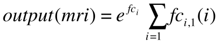 (8)
Dropout regularisation is applied in FC1, FC2 and FC3 to reduce dependence on particular pooling-layer features and improve robustness.
(v) Batch Normalization
ODAN uses learning-rate and layer optimisation to support training performance. Batch normalisation introduces two learnable parameters per activation. The training stage can use mini-batch-dependent activations, while inference should produce outputs determined by the input image. The relationship is expressed below.
 (9)
This expression describes normalisation within the convolutional and fully connected layers using the activation values, learning parameters and bias. The procedure is intended to improve the medical-image representation through normalised learning.
(vi) Optimal Convolution
The final module combines the training objectives through joint optimisation to reduce prediction error. Training a deep network directly can be difficult; suitable initialisation can support stable training and faster convergence. The optimal DAN formulation is expressed below.
 (10)
DAN gives particular attention to image-texture information to support feature learning. The study evaluates network depth and reconstruction performance for medical-image classification [27], considering MCI, AD and NC images.
Results and Discussion
The ADMRI model is implemented in MATLAB 2016a on an i5 processor with 4 GB RAM. A validation set monitors training and helps select model weights. The following subsections describe the dataset, experimental results and classifier comparisons using confusion-matrix measures.
Dataset
The dataset is obtained from ADNI and contains MRI scans acquired with 3 T scanners. Participants are scanned at baseline and at subsequent visits after one, two and three years. The source analysis treats each scan as a separate sample. Figure 6 presents sample images.
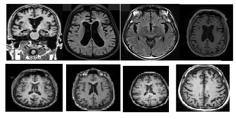
Figure 6: MRI image database
The source reports a total of 355 MRI volumes, alongside class counts of 45 normal controls, 71 MCI cases and 33 AD cases. These reported figures are retained. Data augmentation is applied to smaller classes to balance the multiclass dataset.
Table 1: Pre-processed ADMRI
Input Images | Noise Removal | Filtered images |
|
|
|
|
|
|
|
|
|
|
|
|
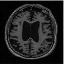
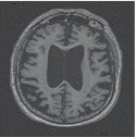
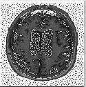
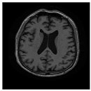
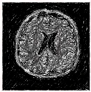
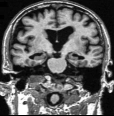
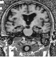
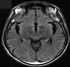
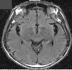
Table 1 presents the input MRI images and their preprocessing outputs, including region-of-interest extraction and noise removal. The source states that T1-weighted scans underwent bias-field inhomogeneity correction as part of ADNI preprocessing before download.
Table 2: Medical images with Stream cipher results
Input image | Cipher image | CPU Time (sec) | Entropy | Security accuracy (%) | Throughput (kbps) |
|
| 111.25 | 7.69 | 93.23 | 3456.8 |
|
| 120.45 | 7.84 | 89.85 | 4521 |
|
| 109.2 | 7.56 | 91.18 | 3546.89 |
|
| 121.89 | 8.02 | 92.33 | 3158 |
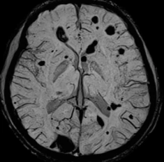
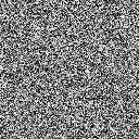
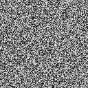
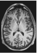
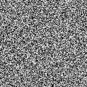
Table 2 presents stream-cipher security results, including the input and encrypted images, processing time, entropy, security accuracy and throughput. The source also reports throughput of 40 Mb, MAE of 0.124 and NPCR of 98.56%. In the character-encoding procedure, characters in the plain-image key sequence are replaced according to the mutated encoding table to support image security.
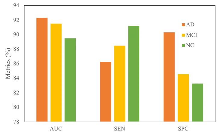
Figure 7: Comparative results based on class
Figure 7 compares classification measures, including accuracy, sensitivity and specificity. The model uses image features to classify MRI scans as AD, MCI or NC. Distinguishing MCI is relevant to research into progression towards AD. The source describes an application that assigns a class after an MRI image is uploaded and proposes stage-related guidance; this remains a research proposal rather than validated clinical advice. It reports values labelled AUC, sensitivity (SEN) and specificity (SPC) of 95.6%, 94.78% and 92.15%, respectively.
Table 3: ADMRI with class for proposed ODAN
Input image | Class | AUC | SPC | SEN |
| AD | 92.2 | 88.56 | 90.2 |
| MCI | 93.22 | 82.25 | 84.2 |
| AD | 89.46 | 87.46 | 92.2 |
| NC | 91.2 | 86.2 | 85.2 |
| MCI | 87.58 | 91.2 | 96.5 |
Table 3 presents example images, predicted classes and performance measures for ODAN. Hyperparameters are selected using training and validation data, while the test set is reserved for evaluation without further learning. The source reports AUC of 96.56%, SEN of 89.56% and SPC of 93.556%. It also compares AlexNet with the optimised version after halving the number of feature maps, reporting an approximately 5% increase in test accuracy after adding a deconvolution layer.
Performance comparison
Accuracy
Sensitivity
Specificity
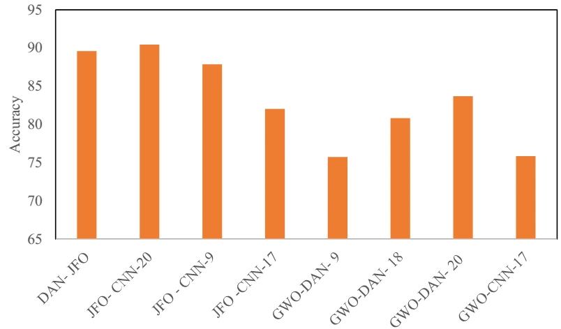
Figure 8: Comparative analysis
Table 4: Summary of Results of Alzheimer detection
Class | Metrics | DAN- JFO | JFO- CNN-20 | JFO – CNN-9 | JFO -CNN-17 | GWO-DAN- 9 | GWO-DAN- 18 | GWO-DAN- 20 | GWO-CNN-17 |
AD | Accuracy | 92.3 | 92.1 | 86.2 | 89.6 | 63.2 | 85.2 | 79.2 | 83.2 |
MCI | 86.25 | 90 | 91.2 | 74.2 | 89.5 | 81.1 | 88.2 | 65.2 | |
NC | 90.3 | 89.2 | 86.2 | 82.3 | 74.5 | 76.2 | 82.290.2 | 79.2 | |
AD | Sensitivity | 91.5 | 85.2 | 96.25 | 69.56 | 79.25 | 79.2 | 79.25 | 82.2 |
MCI | 88.47 | 75.2 | 84.2 | 60.3 | 82.2 | 65.28 | 69.2 | 79.58 | |
NC | 84.56 | 63.2 | 63.2 | 68.2 | 86.2 | 76.28 | 82.5 | 73.54 | |
AD | Specificity | 89.46 | 85.2 | 62.2 | 85.2 | 76.2 | 71.25 | 91.2 | 79.28 |
MCI | 91.2 | 92.2 | 79.2 | 83.2 | 89.2 | 69.23 | 82.2 | 81.59 | |
NC | 83.25 | 73.2 | 72.2 | 73.25 | 90.25 | 67.25 | 80.98 | 83.57 |
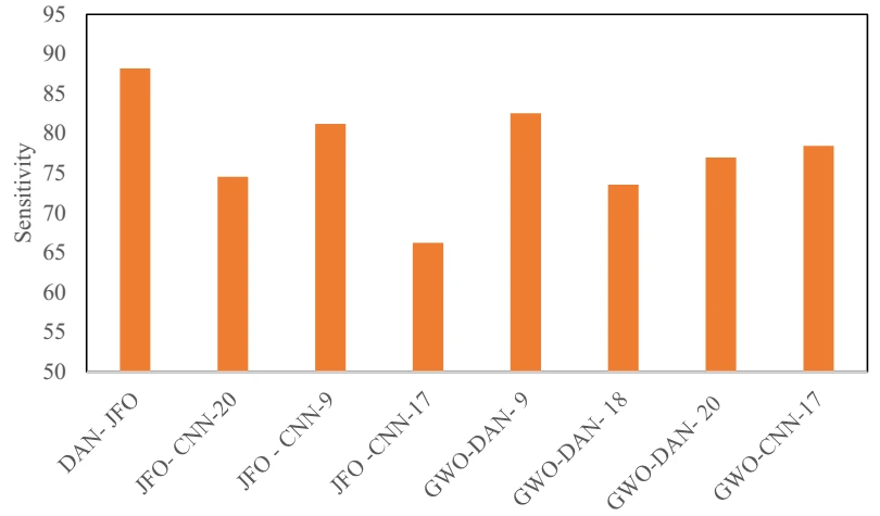
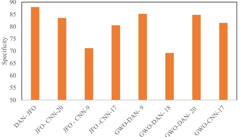
Table 4 and Figure 8 summarise the classification comparison. The source reports improved performance when imaging biomarkers and selected features are combined. Voxel-based features and other biomarkers are extracted from each modality to calculate pairwise similarities. Similarity graphs from the modalities are then combined for multiclass classification. DAN-JFO is reported to improve accuracy by 3.05% relative to GWO-CNN-9, 2.47% relative to JFO-CNN-17, 1.46% relative to GWO-CNN-18, 2.82% relative to JFO-CNN-20, 2.24% relative to JFO-CNN-9, 1.91% relative to GWO-CNN-17 and 2.02% relative to GWO-A*-CNN-20. The study prioritises recall because missed AD cases are an important concern in screening research. These experimental comparisons do not establish clinical diagnostic performance.
Table 5: Quality Results K fold validation
Image | K=5 | K=10 | K=15 | ||||||
I | AUC | SPC | SEN | AUC | SPC | SEN | AUC | SPC | SEN |
2 | 92.22 | 85.2 | 81.2 | 79.65 | 72.22 | 81.23 | 56.22 | 81.2 | 79.25 |
3 | 86.2 | 82.2 | 83.2 | 72.2 | 89.2 | 83.2 | 62.45 | 73.22 | 71.2 |
4 | 85.2 | 89.56 | 90.2 | 73.56 | 91.22 | 79.8 | 63.28 | 62.25 | 82.2 |
5 | 91.2 | 79.4 | 91.28 | 89.56 | 86.25 | 71.25 | 71.2 | 63.9 | 83.6 |
6 | 92.5 | 86.2 | 89.2 | 88.5 | 90.2 | 79.23 | 79.2 | 65.8 | 84.5 |
Table 5 reports classification results for cross-validation settings K = 5, 10 and 15. The source evaluates retrieval speed and the measures labelled AUC, SPC and SEN. Its qualitative assessment suggests that ODAN-JSO produces fewer artefacts and better preserves image structures used to identify abnormal regions.
Table 6: Overall efficiency analysis
Images | Security | Detection-ODAN | DAN | Pooling of AlexNet | Feature maps | Trian/ test |
I1 | 85.2 | 98.2 | 82.2 | 36.2 | 66.3 | 82.2 |
I2 | 81.2 | 92.3 | 78.2 | 53.2 | 69.2 | 63.2 |
II43 | 83.22 | 56.2 | 65.2 | 32.2 | 75.2 | 89.2 |
I5 | 76.2 | 86.2 | 80.2 | 39.2 | 73.2 | 84.5 |
I6 | 82.2 | 81.2 | 73.2 | 46.2 | 65.2 | 92.2 |
I7 | 92.3 | 92.33 | 63.2 | 48.5 | 79.21 | 79.2 |
Table 6 evaluates JSO-based feature selection in AlexNet across three original feature sets. The source compares AD, MCI and NC classification using the reported confusion-matrix measures and records a 50% performance improvement after hyperparameter tuning. The reported values are retained as experimental findings.
Conclusion
This study examines machine-based MRI classification for AD research. Its proposed workflow combines stream-cipher image security with an optimised deep AlexNet classifier and evaluates multiple classes using ADNI data. The source reports accuracy, sensitivity and specificity values of 96.23, 94.55 and 82.2, respectively, for the JSO-CNN classification process. The experimental results are presented as improvements over the compared classifiers, although they do not establish clinical validity or demonstrate improved treatment outcomes. Future work should include additional dementia types and independent validation to assess whether the approach can support clinically useful classification.
References
[1] Balaji, Prasanalakshmi, Mousmi Ajay Chaurasia, Syeda Meraj Bilfaqih, Anandhavalli Muniasamy, and Linda Elzubir Gasm Alsid. “Hybridized Deep Learning Approach for Detecting Alzheimer’s Disease.” Biomedicines 11, no. 1 (2023): 149.
[2] Liu, Siqi, Sidong Liu, Weidong Cai, Sonia Pujol, Ron Kikinis, and Dagan Feng. “Early diagnosis of Alzheimer’s disease with deep learning.” In 2014 IEEE 11th international symposium on biomedical imaging (ISBI), pp. 1015-1018. IEEE, 2014.
[3] Marcolla, Chiara, Victor Sucasas, Marc Manzano, Riccardo Bassoli, Frank HP Fitzek, and Najwa Aaraj. “Survey on Fully Homomorphic Encryption, Theory, and Applications.” Proceedings of the IEEE 110, no. 10 (2022): 1572-1609.
[4] KP, Muhammed Niyas, and P. Thiyagarajan. “Alzheimer’s classification using dynamic ensemble of classifiers selection algorithms: A performance analysis.” Biomedical Signal Processing and Control 68 (2021): 102729.
[5] Kruthika, K. R., H. D. Maheshappa, and Alzheimer’s Disease Neuroimaging Initiative. “Multistage classifier-based approach for Alzheimer’s disease prediction and retrieval.” Informatics in Medicine Unlocked 14 (2019): 34-42.
[6] Feng, Jinwang, Shao-Wu Zhang, Luonan Chen, and Alzheimer’s Disease Neuroimaging Initiative (ADNI. “Identification of Alzheimer’s disease based on wavelet transformation energy feature of the structural MRI image and NN classifier.” Artificial Intelligence in Medicine 108 (2020): 101940.
[7] Shankar, K., S. K. Lakshmanaprabu, Ashish Khanna, Sudeep Tanwar, Joel JPC Rodrigues, and Nihar Ranjan Roy. “Alzheimer detection using Group Grey Wolf Optimization based features with convolutional classifier.” Computers & Electrical Engineering 77 (2019): 230-243.
[8] Singh, Simarjeet, and Rekh Ram Janghel. “Early diagnosis of alzheimer’s disease using aco optimized deep cnn classifier.” In Ubiquitous Intelligent Systems: Proceedings of ICUIS 2021, pp. 15-31. Springer Singapore, 2022.
[9] Jia, Hongfei, Yu Wang, Yifan Duan, and Hongbing Xiao. “Alzheimer’s Disease Classification Based on Image Transformation and Features Fusion.” Computational and Mathematical Methods in Medicine 2021 (2021).
[10] Altaf, Tooba, Syed Muhammad Anwar, Nadia Gul, Muhammad Nadeem Majeed, and Muhammad Majid. “Multi-class Alzheimer’s disease classification using image and clinical features.” Biomedical Signal Processing and Control 43 (2018): 64-74.
[11] Beheshti, Iman, Hasan Demirel, and Alzheimer’s Disease Neuroimaging Initiative. “Feature-ranking-based Alzheimer’s disease classification from structural MRI.” Magnetic resonance imaging 34, no. 3 (2016): 252-263.
[12] Farhan, Saima, Muhammad Abuzar Fahiem, and Huma Tauseef. “An ensemble-of-classifiers based approach for early diagnosis of Alzheimer’s disease: classification using structural features of brain images.” Computational and mathematical methods in medicine 2014 (2014).
[13] Divya, R., R. Shantha Selva Kumari, and Alzheimer’s Disease Neuroimaging Initiative. “Genetic algorithm with logistic regression feature selection for Alzheimer’s disease classification.” Neural Computing and Applications 33, no. 14 (2021): 8435-8444.
[14] Lu, Bin, Hui-Xian Li, Zhi-Kai Chang, Le Li, Ning-Xuan Chen, Zhi-Chen Zhu, Hui-Xia Zhou et al. “A practical Alzheimer’s disease classifier via brain imaging-based deep learning on 85,721 samples.” Journal of Big Data 9, no. 1 (2022): 1-22.
[15] Hajamohideen, Faizal, Noushath Shaffi, Mufti Mahmud, Karthikeyan Subramanian, Arwa Al Sariri, Viswan Vimbi, and Abdelhamid Abdesselam. “Four-way classification of Alzheimer’s disease using deep Siamese convolutional neural network with triplet-loss function.” Brain Informatics 10, no. 1 (2023): 1-13.
[16] Chen, Yuanyuan, and Yong Xia. “Iterative sparse and deep learning for accurate diagnosis of Alzheimer’s disease.” Pattern Recognition 116 (2021): 107944.
[17] Singh, Simarjeet, and Rekh Ram Janghel. “Early diagnosis of alzheimer’s disease using aco optimized deep cnn classifier.” In Ubiquitous Intelligent Systems: Proceedings of ICUIS 2021, pp. 15-31. Springer Singapore, 2022.
[18] Priyanka Nedunchellian, Ahana, and Kavitha Ganesan. “Study of onset in brain dementia using hierarchical wolf colony optimization and dual deep learning technique.” The Imaging Science Journal 70, no. 3 (2022): 155-167.
[19] Shaji, Sreelakshmi, Jac Fredo Agastinose Ronickom, Anandh Kilpattu Ramaniharan, and Ramakrishnan Swaminathan. “Study on the effect of extreme learning machine and its variants in differentiating Alzheimer conditions from selective regions of brain MR images.” Expert Systems with Applications 209 (2022): 118250.
[20] Garg, Neha, Mahipal Singh Choudhry, and Rajesh M. Bodade. “A review on Alzheimer’s Disease Classification from Normal Controls and Mild Cognitive Impairment using structural MR Images.” Journal of Neuroscience Methods (2022): 109745.
[21] De Mendonça, Lucas José Cruz, Ricardo José Ferrari, and Alzheimer’s Disease Neuroimaging Initiative. “Alzheimer’s disease classification based on graph kernel SVMs constructed with 3D texture features extracted from MR images.” Expert Systems with Applications 211 (2023): 118633.
[22] Helaly, Hadeer A., Mahmoud Badawy, and Amira Y. Haikal. “Deep learning approach for early detection of Alzheimer’s disease.” Cognitive computation (2021): 1-17.
[23] Mehmood, Atif, Muazzam Maqsood, Muzaffar Bashir, and Yang Shuyuan. “A deep Siamese convolution neural network for multi-class classification of Alzheimer disease.” Brain sciences 10, no. 2 (2020): 84.
[24] Zheng, Jun, and Hanping Hu. “A highly secure stream cipher based on analog-digital hybrid chaotic system.” Information Sciences 587 (2022): 226-246.
[25] Li, Gordon HY, Ryoto Sekine, Rajveer Nehra, Robert M. Gray, Luis Ledezma, Qiushi Guo, and Alireza Marandi. “All-optical ultrafast ReLU function for energy-efficient nanophotonic deep learning.” Nanophotonics (2022).
[26] Sun, Yongjian, and Shaohui Li. “Bearing fault diagnosis based on optimal convolution neural network.” Measurement 190 (2022): 110702.
Cite This Work
To export a reference to this article please select a referencing stye below:

Academic Master Education Team is a group of academic editors and subject specialists responsible for producing structured, research-backed essays across multiple disciplines. Each article is developed following Academic Master’s Editorial Policy and supported by credible academic references. The team ensures clarity, citation accuracy, and adherence to ethical academic writing standards
Content reviewed under Academic Master Editorial Policy.