Alzheimer MRI Classification with Fused Features and Osprey Badger Optimisation

Abstract

In order to improve the classification and segmentation of MRI scans for Alzheimer’s disease (AD), a novel metaheuristic-driven approach is introduced in this study. The research framework comprises four pivotal phases, commencing with data acquisition from an open-access online repository, with a dataset spanning four distinct AD classes. Modern methods are used to improve the quality of the MRI images, including local entropy-weighted histogram equalisation made possible by the adaptive-wind-driven-optimization (AWDO) algorithm. Furthermore, guided filter-based image denoising is implemented and strengthened by the performance of an adaptive-salp-swarm-optimization (ASSO) algorithm. The core of this approach harnesses the power of deep learning, employing a ResNet152-based model for spatial feature extraction, with the omission of the final classification layer. The segmentation process adopts Otsu’s thresholding, refined through the novel Osprey Badger optimization (OBO) algorithm, synergizing aspects of the Osprey optimization algorithm (OOA) and Honey Badger algorithm (HBA) to achieve optimal thresholding and highly efficient segmentation. The feature extraction phase is equally comprehensive, encompassing gray-level co-occurrence matrices (GLCM), texture features (Mean, Variance, and entropy), and Edge Features using the Canny edge detection method, and scale-invariant feature transform (SIFT) features, strategically concatenated with the ResNet152 (Residual Networks) features, enriching the feature representation. This amalgamation of multifaceted features significantly strengthens the classification process, with densely connected Gated Recurrent Unit (DGRU) leveraged for advanced AD classification.

Keywords: Alzheimer’s disease; OOA; HBA; OBO; DGRU; ResNet152.

Introduction

AD is a fatal and progressive neurodegenerative condition that presents a serious threat to world health. It is the most prevalent type of dementia and is characterized by a slow decline in cognitive function, memory loss, behavioral abnormalities, and difficulty carrying out daily tasks [1,2]. The prevalence of AD is anticipated to significantly rise as the world’s population ages, making it an urgent public health problem [3]. For a number of reasons, such as giving patients access to prospective therapies, enabling carers to make future plans, and facilitating research into the creation of efficient interventions, an early and precise diagnosis of AD is essential [4]. AD not only affects individuals diagnosed with the disease but also places an enormous emotional, psychological, and financial burden on their families and society as a whole [5,6]. It is estimated that more than 50 million people worldwide are living with dementia, and AD accounts for approximately 60-70% of these cases. The global cost of dementia care was estimated at around $1 trillion in 2018, a figure expected to double by 2030. These statistics underscore the urgent need for effective strategies in AD detection and management [7]. One of the significant challenges in addressing AD is the difficulty of diagnosing the disease accurately and at an early stage [8].

AD is a complex condition with a long preclinical phase during which pathological changes are occurring in the brain, but symptoms are not yet evident [9,10]. By the time clinical symptoms become apparent, significant brain damage may have already occurred, making interventions less effective [11]. Therefore, there is a critical need to develop methods for detecting AD in its earliest stages, ideally before cognitive decline becomes noticeable. While these methods remain essential for evaluating patients, they are not sufficient for early and accurate AD detection [12,13]. Neuroimaging techniques have revolutionized our understanding of AD and have emerged as powerful tools for early diagnosis and monitoring. These technologies enable researchers and clinicians to visualize amyloid plaques, tau tangles, and structural brain abnormalities associated with AD. Importantly, they can provide valuable information about brain changes before symptoms appear, offering a window of opportunity for early intervention [14,15]. Recent advances in machine learning and artificial intelligence (AI) have opened up new possibilities for AD detection and diagnosis. These technologies can analyze vast amounts of neuroimaging and clinical data with a level of precision and speed beyond human capabilities. The goal of this research is to develop more precise and effective diagnostic techniques for AD, a neurodegenerative disorder that has a serious global impact. Traditional diagnostic techniques frequently don’t have the sensitivity needed for early discovery, and incorrect diagnoses might postpone crucial interventions. The combination of deep learning methods like ResNet152 with sophisticated segmentation techniques like OOA and HBA has the potential to improve the precision of AD detection and the effectiveness of the diagnostic procedure. By leveraging multiple levels of fused features, including spatial, textural, and edge features, this approach aims to significantly improve the classification of AD, potentially leading to earlier intervention and improved patient outcomes.

The primary contribution of this research work is:

To improve feature extraction, a ResNet152-based model is employed, focusing on spatial features while disregarding the final classification layer.

To enhance image segmentation, the framework adopts Otsu’s thresholding and refines it with an OBO algorithm, providing an optimal threshold for more efficient segmentation.

To enrich feature representation, the framework leverages a combination of techniques, including GLCM, Texture features, Canny edge detector, and SIFT features.

To boost classification accuracy, the extracted features are concatenated with the ResNet152 features, creating a multi-feature representation.

To further improve classification, the concatenated features are input into densely connected GRU, facilitating better Alzheimer’s disease classification.

The remaining sections are organised as follows: Section 2 discusses the studies and reviews of the literature that are pertinent to the subject. In Section 3, the suggested framework is discussed. The results are discussed in Section 4 and the study is concluded in Section 5.

Literature Review

AD and its early stage, moderate cognitive impairment (MCI), present considerable obstacles for early identification in 2022, according to Odusami et al. [16]. For this reason, deep learning techniques have gained popularity. These algorithms, however, frequently have trouble spotting modifications in the functional connectivity of MCI patients’ brain networks. A study that addressed this issue classified AD by combining deep features from two already-trained models, ResNet18 and DenseNet201.

According to Puente-Castro et al. [17] in 2020, early diagnosis of AD is crucial for effective treatment. The research proved that it is possible to identify AD-related damage and stages in sagittal MRIs by using Transfer Learning (TL) approaches. Sagittal MRI results were important since they were equivalent to those from traditional horizontal-plane MRIs, offering up new opportunities for efficient research. This study emphasizes the utility of DL models and TL in sectors with resource-intensive data collecting.

In 2019, timely treatment and the maintenance of essential functions depend on the early diagnosis of brain diseases, according to Talo et al. [18]. Manually identifying brain abnormalities in MRI scans may be challenging, particularly early on. This work used deep learning models including AlexNet, Vgg-16, ResNet-18, ResNet-34, and ResNet-50 to classify MR images into various disease classes. The ResNet-50 model got the highest classification accuracy (95.23% 0.6).

AD is a prevalent yet frequently misdiagnosed form of dementia that has no known cure as of 2019, according to Kruthika et al. [19]. Effective management requires early identification of moderate cognitive impairment (MCI). Increased diagnostic accuracy is possible with content-based image retrieval (CBIR) systems and machine learning classifiers like SVM, Naive Bayes, and K-nearest neighbor (KNN). In this study, feature selection was accomplished using particle swarm optimization (PSO) on MRI images that had been processed using FreeSurfer.

Effective medical categorization frequently necessitates diverse multi-modal data and the capacity to handle multiple feature kinds, according to Liu et al. in 2023 [20]. Existing models are excellent at using data from several modalities, but they struggle with missing modalities and frequently discard samples, which hinders data-driven techniques like deep learning. To solve this by introducing the Multi-Modal Mixing Transformer (3MT), which enables robust management of missing data in addition to multi-modal data integration. 3MT uses a Cascaded Modality Transformers design with cross-attention and a unique modality dropout mechanism that has been tested on AD and CN categorization and MCI conversion prediction.

Early identification of AD remains difficult in 2020, but deep convolutional neural networks (CNN) have showed potential in brain image analysis, according to Mehmood et al. [21]. A crucial tool for diagnosing AD is magnetic resonance imaging (MRI), but the lack of sufficient image data can cause deep learning models to overfit. We created a Siamese CNN model based on VGG-16 to handle this issue while augmenting the data with augmentation methods.

According to AbdulAzeem et al. [22] in 2021, increasing relevance of healthcare innovations is obvious in boosting longevity and general well-being, especially in tackling AD. Due to the substantial caregiving costs associated with AD, a common neurodegenerative illness, a timely and precise classification method is essential. With its advantages over conventional machine learning, deep learning has becoming more popular. CNN and brain MRI images have been used in recent research that have showed promise in the diagnosis of AD.

The prediction of AD by Basheera and Ram [23] based on mild cognitive impairment (MCI) and cognitive normality (CN) has received a lot of attention in 2020. Recent developments in neuroimaging and machine learning provide useful instruments for the early AD diagnosis. It is still difficult to tell the difference between healthy atrophy and early pathological brain atrophy. This work offers a model for better MCI and CN distinction, aiding in the early diagnosis of AD.

A new deep ensemble learning framework for categorizing AD is introduced in a publication by An et al. [24] in 2020, utilising the strength of deep learning algorithms and multisource data integration. In order to learn features and increase variety among base classifiers, the framework uses two sparse autoencoders at the voting layer. To rank base classifiers, the stacking layer uses a nonlinear feature-weighted approach based on a deep belief network. The meta-classifier is a neural network. By utilising threshold-moving and oversampling approaches, the optimizing layer tackles challenges that are cost-sensitive. This novel method improves the detection and treatment of AD by utilising the collective machine learning skills.

According to Fan et al. [25], AD is a typical neurologic disease that leads to dementia and memory loss in 2020. The prevalence of AD has elevated to the level of a serious health concern. Along with cancer, cardiovascular disorders, and cerebrovascular diseases, AD poses a serious health risk to the elderly with an estimated average survival time of about 5.5 years. This study uses support vector machine (SVM) models with structural brain MRI data to categorize and forecast different phases of AD, assisting in disease diagnosis, in order to address this pressing issue. Table 1 presents the identified research gaps in existing studies.

Table1: ResearchGaps

ProposedMethodology

AD is a progressive neurological disorder marked by cognitive decline and brain abnormalities. Precise segmentation and classification of AD are complex due to symptom variations, necessitating early diagnosis. This study introduces a deep learning-based framework for AD detection, focusing on improving segmentation and classification accuracy. The model comprises four phases: data collection, pre-processing, segmentation, feature extraction, and classification, as illustrated in Figure 1.

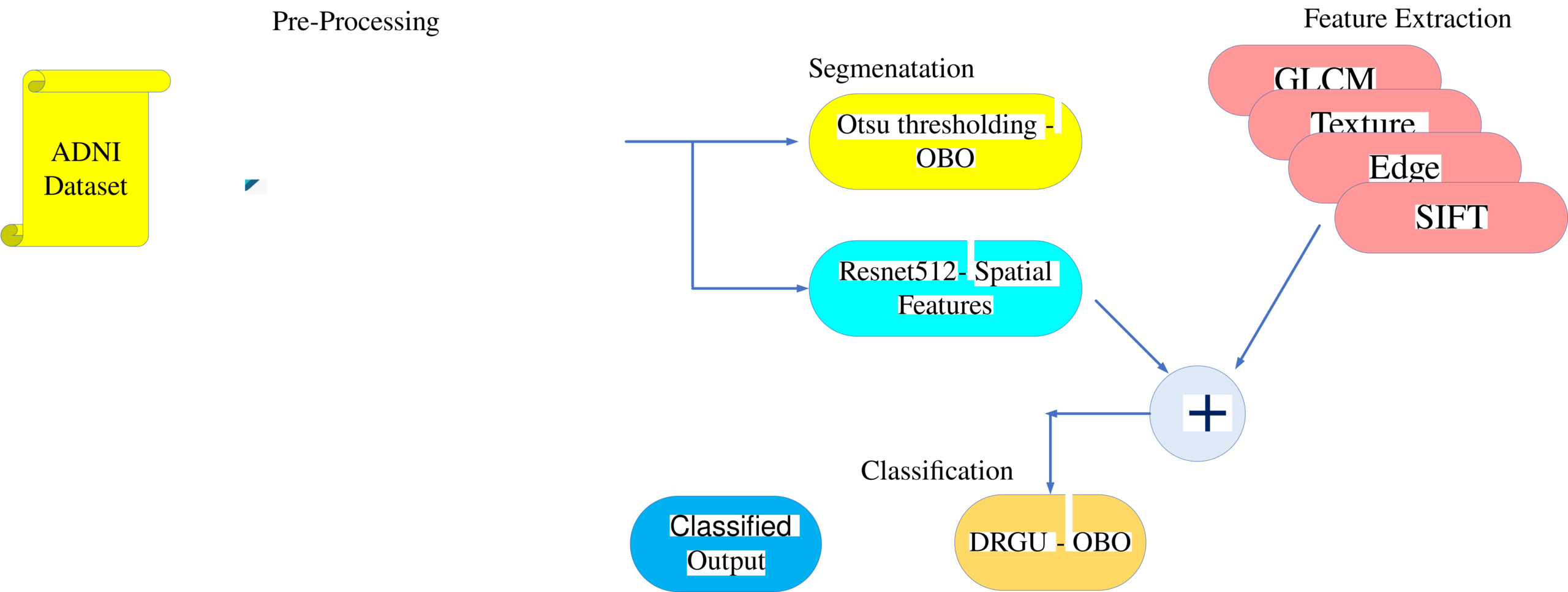
Figure 1: Overall Proposed Architecture

Dataset Description

The Alzheimer’s Disease Neuroimaging Initiative (ADNI) dataset [27] is a long-term study focused on early Alzheimer’s Disease (AD) detection and progression monitoring. This dataset comprises 2D axial images derived from the original ADNI dataset, initially containing Nifti images. It encompasses three classifications: AD, Mild Cognitive Impairment (CI), and Common Normals (CN). AD is a progressive disease affecting memory, reasoning, and behavior. CI involves memory and cognitive issues without significant daily life interference. CN represents individuals without dementia or cognitive impairment. Researchers widely employ the ADNI dataset to develop and evaluate machine learning models for early AD identification and diagnosis. The dataset has shown to be a beneficial tool for creating forecasting models and locating biomarkers that could help identify people at risk of developing AD. The dataset comprises a total of 5,154 images. To form the training set, 80% of these images, which corresponds to 4,123 images, are designated for training purposes. The remaining 20% of the image dataset, totalling 1,031 images, is set aside for testing and evaluation. This partitioning into training and testing sets follows standard procedures in machine learning to assess model performance and generalization.

Pre-Processing

In this study, preprocessing involves several key steps. These methods encompass local entropy-weighted histogram equalization with AWDO, guided filter-based image denoising optimized using ASSO, imageaugmentation, geometrictransformations, noisereduction, and grayscaleconversion.

Enhanced Histogram Equalization with Local Entropy

Local Entropy Weighted Histogram Equalization is a valuable technique for enhancing the clarity of MRI brain images in Alzheimer’s disease detection. It divides images into sub-regions, equalizes their histograms independently, and uses local entropy for weighting. This improves image quality and aids AD detection efficiently. The algorithm involves dividing the image, calculating local entropy, creating local entropy-weighted histograms, segmenting, equalizing, and reconstructing the final image. The best threshold, designated as a_I^*, is discovered by exhaustively seeking the interclass variance maximum generated by Eq. (1) and Eq. (2).

0 < a_I< L-1 (1)

argmax{σ_aI²} = a_I (2)

Where, L is grayscale number in the image, and σ_aI² is interclass variance as per Eq. (3).

σ_aI² = w_B(I)w_F(I)[μ_B(I) – μ_F(I)]² (3)

where w_B(I), w_F(I) represents the back ground, fore ground classes, respectively, and μ_B(I) and μ_F(I) denotes means. These parameters can be calculated using Eq. (4) to Eq. (7).

w_B(I) = ∑_s=0^a(p(I_s)) (4)

w_F(I) =∑_s=a+1^L-1(p(I_s)) (5)

μ_B(I) =(∑_s=0^a(p(I_s)).s)/(W_B(I)) (6)

μ_F(I) = (∑_s=a+1^L-1(p(I_s)).s)/(W_F(I)) (7)

where p(I_s) is the likelihood that the histogram’s sth grayscale level will appear. The final improved image is created by combining the two sub-images. For each sub-histogram, the grayscale transfer functions a_I^*can be determined using Eq. (8) and Eq. (9).

*A(I) = (I – I_min) * (En_k – En₀) / (a * (L-1)) + En₀, for 0 <= I <= a (8)

*A(I) = ( I_max – I) * (En_L-1 – En_a) / ((L-1-a) * (L-1)) + En_a, for a< I <= L-1 (9)

where I_min and I_max are the image’s minimum and maximum grayscale values, En₀, En_t, and En_L-1 denotes cumulative entropy values at grayscale levels 0, a, and L-1. En_k represents total entropy of the kth subhistogram.

AWDO

To determine the optimal threshold for Alzheimer’s detection, employ the AWDO algorithm, enhancing image quality for disease detection. AWDO, inspired by wind gust behavior, efficiently searches for the ideal threshold. Combining these approaches improves Alzheimer’s diagnosis. AWDO, derived from nature, leverages air parcel movement in the atmosphere, enhancing WDO’s performance with adaptive mutation rates and crossover probabilities. This versatile algorithm has successfully tackled optimization challenges in various fields, with distinct phases and procedures. The algorithm starts by initializing parameters like population size, iterations, search space bounds, mutation rate, and crossover probability. Next, it assesses air parcel pressures based on the objective function using Eq. (10).

P = (y – l)/(u – l) (10)

When y denotes the air parcel’s present location, u denotes the search space’s upper bound, and l denotes its lower bound.

During adaptive mutation and crossover phase, the algorithm adjusts the mutation rate and crossover probability according to population performance in previous iterations using Eq. (11) and Eq. (12).

P(i) = P(i-1) × c (11)

R(i) = R(i-1) × d (12)

Where P(i) and R(i) represent the adaption rates at iterations i, c, and d and P(i-1) and R(i-1) represent the mutation rate and crossover probability in the preceding iteration. In Mutation Operation Phase, new air parcels are created by applying mutation and crossover operations to the current population.

M(i+1,j) = M(i,j) + P(i) × (Y(i,j) – Y(i,k)) (13)

where Y(i,j) and Y(i,k) are two randomly chosen air parcels from the population in iteration i, M(i+1,j) is the new location of air parcel j in iteration i+1, M(i,j)is the current position of air parcel j in iteration i, and P(i) is the mutation rate in iteration i. In the Selection Phase, the algorithm chooses the next population based on current performance, utilizing a roulette wheel selection method. In the Termination Phase, the algorithm stops when predefined criteria are met.

GuidedFilter-ImageDenoising

The adaptive guidance image considers the image’s structure and features, guiding the filtering process to preserve edges and textures while reducing noise. According to Eq. (14) the guided filter’s output is provided.

D(x,y) = (1/|w|) * ∑(x,y)∈w [W(x,y)*g(x,y)*N(x,y)] (14)

In this equation, D represents the denoised image, (x, y) pixel indices, W kernel weights linearly varying with noisy image N guided by image g, and w filter window.

D(x,y) = a_s*g(x,y) + b_s (15)

Here, (a,b) are presumed constant linear coefficients within window ws, and ε is the regularization parameter controlling smoothing. Linear regression minimizes the window’s cost function, determining a_s and b_s values using Eq. (16) and Eq. (17).

a_s= |(1)/(|w|)|* ∑_x,y∈ws(g_x^°N-μ_sN)/σ_s²+γ_s²+ε (16)

b_s = N-a_sμ_sγ_s (17)

Here, μ_sN, σ_s², and γ_s² denote the noisy image 𝑁’s mean, variance, and skewness within window ws. The filter kernel weights W(x,y) ensure unit summation and are defined by Eq. (18).

W(x,y) (g)= (1/|w|²) * ∑_s:x,y∈ws([(1 + (G(x)- μ_s)(G(y)- μ_s))/(σ_s²+γ_s²+ε)]) (18)

In the window ws, μ_s and σ_s² of the guidance image are significant. A regularization parameter controls smoothing and feature preservation in noisy regions. ASSO inspired by salps’ behavior and adaptation, optimizes image features.

ASSO

ASSO, a derivative of SSO, harnesses salp-inspired optimization techniques to enhance image feature selection. This algorithm, tailored for AD classification, introduces the concept of inertia weight. The inertia weights, adjusted dynamically with iteration number, aim to optimize the balance between local exploitation and global exploration. In ASSO, the leader’s position update equation from the SSO algorithm undergoes modification as per Eq. (19).

x_j¹={w*A_j+v₁((UB_j-LB_j)v₂+LB_j) v₃≥0 ; w*A_j-v₁((UB_j-LB_j)v₂+LB_j) v₃<0 (19)

ASSO algorithms employ a strategy for inertia weights w, specifically the non-linear coefficient decreasing inertia weight ASSO-NLDIW. In each iteration, the value of 𝑤 is evaluated according to Eq. (20).

wt = wmax – (wmax – wmin) * ((t)/(T))^u (20)

where wmin and wmax are set to 0 and 2, respectively, and parameter u is set to u = 1/π².

Geometrictransformations

Geometric transformations play a crucial role in the pre-processing of medical images for AD segmentation and classification. These transformations involve spatial adjustments of image pixels to enhance image quality, improve contrast, or aid in region-specific segmentation. Translation shifts an image in a chosen direction, aligning images captured from different angles. Reflection flips an image horizontally or vertically, correcting lighting and angle variations. Rotation rotates an image around a point to rectify oblique captures. Dilation, a morphological operation, alters object sizes by adding or removing pixels, useful for feature enhancement and noise reduction. Adjusting the structuring element’s size and shape customizes the effect in AD image pre-processing.

ImageAugmentation

Image augmentation is a critical technique in preprocessing images for AD detection. Its main goal is to expand the training dataset by generating diverse images from the originals, reducing overfitting, and improving the model’s generalization. Strategies include rotation, flipping, zooming, cropping, and adding Gaussian noise. Rotation adds new angles, flipping mirrors images, zooming provides different perspectives, cropping focuses on various regions, and Gaussian noise varies noise levels. These techniques enrich the training dataset, helping the AD detection model adapt to a wider range of scenarios and variations in medical imaging data.

NoiseReduction

Image denoising is a crucial step in AD diagnosis from MRI images, focusing on improving image quality and enhancing the signal-to-noise ratio (SNR). Various techniques are available, including linear and nonlinear filters. Linear filters like mean, median, and Gaussian filters are efficient but can blur edges. Mean replaces pixel values with the average of neighbours, suitable for low SNR. Median is nonlinear, excelling in impulsive noise reduction while preserving edges. Gaussian filters are effective against correlated noise but may blur edges, depending on kernel size. Nonlinear methods like Total Variation (TV) and Non-local Means (NLM) filters effectively reduce noise while preserving details, with NLM being computationally efficient and widely used in medical imaging, including MRI and CT scans.

Grayscale Conversion

Grayscale conversion is a common pre-processing technique in medical image processing, particularly in AD diagnosis. Grayscale images consist of varying shades of gray, with black as the lowest intensity and white as the highest. This conversion involves transforming a color image into grayscale, retaining only the luminance or brightness data. Grayscale images simplify computational tasks, preserve structural information, and save memory space. In AD diagnosis, grayscale brain images are used to detect abnormalities like atrophy and lesions. Typically, grayscale conversion is the first step before further image analysis techniques, such as segmentation and feature extraction, are applied to aid in diagnosis.

Segmentation

Otsu’s thresholding method is employed for segmentation, and it is enhanced using an innovative approach involving the integration of OOA and HBA Algorithm. This amalgamation, known as OBO, significantly enhances the efficiency of threshold selection. By leveraging the OBO, the algorithm determines an optimal threshold for Otsu’s method, resulting in highly efficient image segmentation.

Otsu Thresholding

Otsu thresholding is a technique used to automatically determine the optimal threshold for image segmentation by analyzing the image histogram. The histogram provides information about pixel intensities distribution in image. Finding a threshold, designated as “t,” that effectively divides the image into two classes is the objective: O₀ and O₁. O₀ contains pixels with intensities ranging from 0 to t-1, while O₁ contains pixels with intensities from t to the maximum intensity level, typically 255 in grayscale images. The objective is to find ‘t’ such that it maximizes the between-class variance, effectively distinguishing objects or regions of interest from the background as per Eq. (21).

q_i=(n_i)/(N),q_i≥0, ∑_i=0^L(q_i=1) (21)

When a single threshold is applied to an image histogram, it results in the creation of two distinct classes of light intensity. Each of these classes has its own total frequency, which can be denoted as “total frequency left” and “total frequency right” as shown in Eq. (22) and Eq. (23) respectively. The left side and the right side of the threshold represent different regions of the image. The sum of the pixels on both sides of the threshold, as expressed in equation (24), adds up to a total of one.

we₀=∑_i=0^t-1(q_i) (22)

we₁=∑_i=t^L-1(q_i) (23)

we₁=∑_i=t^L-1(q_i) (24)

In the following phase, the total weight of both sides of the threshold, denoted by we₀ and we₁, can be used to determine the average weight of each side of the threshold by computing the total frequency of each light intensity in the two classes around the threshold. q_i is assumed to be determined using Eq. (25) and Eq. (26).

μ₀=∑_i=0^t-1((i∙q_i)/(we₀)) (25)

μ₁=∑_i=t^L-1((i∙q_i)/(we₁)) (26)

The average weights of the light intensity on the left and right thresholds are represented in this equation by μ₀ and μ₁, respectively. Eq. (27) can be used to calculate the average weights of the threshold’s two sides added together. According to Eq. (28), the objective function can be described as the difference between the average values of weights on each side of the threshold and average light intensities.

μ_t=we₀∙μ₀+we₁∙μ₁ (27)

of=we₀∙(μ₀-μ_t)²+we₁∙(μ₁-μ_t)² (28)

Otsu’s approach chooses the right thresholds in an effort to maximize the target’s worth. In this situation, all thresholds must be taken into account. If there are too many thresholds, the Otsu’s processing time will be too long and it won’t be useful.

OBO

A hybrid optimization algorithm, merging the robust foraging persistence of the HBA [27] and the swift, efficient prey detection abilities of the OOA [28], offers a unique approach to problem-solving. This hybrid optimizer blends the patience and tenacity of the HBA with the keen sensory-driven tactics of the HBA. The result is an algorithm that systematically explores solution spaces while swiftly homing in on promising areas. This synergy creates a versatile optimizer capable of tackle a wide range of optimization tasks efficiently and effectively. The OBO algorithm incorporates these behaviors to solve optimization problems.

Mathematical model

The “digging phase” and the “honey phase,” which make up HBA, are separated into the following descriptions. This section presents the proposed HBA algorithm’s mathematical formulation. Since it incorporates both the exploration and exploitation phases, HBA is theoretically a global optimisation technique. Population of potential solutions in HBA is provided by Eq. (29).

inhabitants of candidate [y₁₁ y₁₂ y₁₃ …….. y_1D ; y₂₁ y₂₁ y₂₃ ……… y_2D ; … … … …. ; y_n1 y_n2 y_n3 …….. y_nD] (29)

i^th role of the honey badger y_i=[y_i¹,y_i²,…….,y_i^D]

Step 1: Initialization phase

Calculate the population size (PS) according to Eq. (30), and initialise the number of honey badgers and their locations.

y_i=lob_i+ ra₁*(upb_i-lob_i), ra₁ is a random number between 0 and 1 (30)

where y_i denotes the ith candidate solution in a population of PS, and lob_i and upb_i denote the lower and upper bounds of the search domain, respectively.

Step 2: Fitness calculation – Fitness computation in OBO algorithm involves evaluating the fitness function for each individual in the population, quantifying the performance or quality of their solutions to the problem at hand. The fitness function can be a mathematical formula, simulation, or any other measure specific to the problem, guiding the optimization process towards finding better solutions. It is calculated as per Eq. (31).

fit=min⁡(loss) (31)

Step 2: Updating the agents’ positions

The HBA position update process has two steps, the “digging phase” and the “honey phase” (y_new). The following explains it better:

Step 2-1: Digging phase [proposed]

In this mode, the algorithm seamlessly integrates the honey badger’s capabilities to locate the target’s position, mimicking its hunting behavior. Once in proximity to the target, the honey badger transitions into its characteristic digging phase. This phase combines the position identification and fish hunting behavior inspired by the osprey algorithm with the honey badger’s digging strategy. To optimize the honey badger’s movements, a new position is computed using the proposed Eq. (32), ensuring effective target capture while solving complex problems.

y_i,j¹=y_i,j∙y_pry+ra_i,j∙(sb_i,j-S_i,j.y_new) (32)

Where, y_pry is the location of the target, y_i,j¹ represents the new position of the ith osprey with j dimension based on the first phase of OOA, sb_i,j is the selected fish for ith osprey with its jth dimension, S_i,j are the random numbers from set {1,2}, ra_i,j represents the random numbers in [0,1].

Step 2-2: Honey phase [proposed]

In honey mode, the algorithm emulates the honey badger’s cooperative behavior with the honeyguide bird, leveraging its guidance to locate honey beehives. This phase is then seamlessly integrated with the osprey algorithm’s fish-carrying phase, where the badger’s task shifts from hunting to transporting prey to a suitable location. During this phase, the new position of the ith osprey, characterized by j dimensions, is determined based on the second phase of the OOA. This hybrid approach combines intelligent behaviors from both animals to enhance optimization processes. The scenario in which a honey badger follows a honey guide bird to a beehive can be modelled as per proposed Eq. (33).

y_i,j²=y_i,j+(lob+ ra_i,j∙(upb-lob))/(t) (33)

Where y_i,j² represents the new position of the ith osprey with j dimension based on the second phase of OOA, ra_i,j represents the random numbers in [0,1], t denotes the iterations, upb, lob are the upper bound and lower bound of the jth problem variable respectively, these proposed equations allowing the honey badger to adapt its search strategy and efficiently navigate towards the target location.

Step 4: Termination – The OBO algorithm continues iterating through the search, update, and evolution stages until a certain termination condition is met. This condition can be a predefined number of iterations, reaching a desired fitness level, or the convergence of solutions. Once the termination condition is satisfied, the process is terminated, and the algorithm concludes its execution.

Feature Extraction

In this study, various image features were extracted to enhance AD detection. These included the GLCM, texture features such as mean, variance, and entropy, edge features were obtained using the Canny edge detector to highlight image edges, SIFT, and ResNet152 features were extracted.

GLCM

Texture is one of the most important factors in locating objects or interesting areas in an image. The gray-level co-occurrence matrix or GLCM for short, is a statistical method for analysing texture that takes into account the spatial relationship between pixels. The GLCM functions calculate the frequency of occurrence of pairs of pixels with specific values and in a specific spatial relationship in an image, resulting in a GLCM. From this matrix, statistical measures are then extracted to describe the texture of an image. GLCM serves as the basis for the Haralick texture features.

The C_o number of grey levels in the image is indicated by the dimension C_o of this square matrix. The matrix’s element [d,f] is produced by calculating the total number of times a pixel with value d is next to a pixel with value f, then dividing that number by the total number of times the comparisons were made. Therefore, each entry is taken to represent the likelihood that a pixel with value d will be found close to a pixel with value f. Eq. (34) shows the gray-level co-occurrence matrix.

NG=[ps(1,1) ps(1,2)………ps(1,C_o) ; ps(2,1) ps(2,2)………ps(2,C_o) ; . . …… . ; . . …… . ; ps(C_o,1) ps(C_o,2)………ps(C_o,C_o)] (34)

Texture Features

Mean: Theoretically, mean is defined as the total number of elements divided by the total number of elements in a set. Calculating the mean gives us a good understanding of the entire set of data. Consequently, the mean formula is calculated as per Eq. (35) and Eq. (36).

Mean=(Sum of all the elements)/(Number of elements) (35)

X ̅= (∑(x))/(n) (36)

Where, X ̅= mean value, x = Items given, n = Total number of items

The significance of mean resides in its capacity to sum up the entire dataset in a single value.

Median: The median of a dataset is its midway value. Therefore, the middle value will be the set’s median if a set has an odd number of values. As per Eq. (37), the median will be the average of the two middle values if the set contains an even number of sets.

Median= {(l+1)/(2), for odd ; (l)/(2), for even (37)

Thus, a set of data can be divided into two sections using the median. It is necessary to arrange the set’s components in ascending order in order to determine the set’s median. Then locate the midpoint.

Entropy: Entropy, which is a statistical measure of irregularity or randomness within a dataset. When applied to images, entropy measures the level of variation or unpredictability in the pixel values. Images with highly regular and repetitive patterns, have low entropy because the pixel values are predictable and repetitive. Images with complex and irregular textures, have higher entropy because the pixel values vary more unpredictably. Entropy is calculated by examining the distribution of pixel values in an image. It quantifies the amount of information or uncertainty associated with those values. A high entropy value indicates that the image contains diverse and unpredictable textures, while a low entropy value suggests a more uniform and repetitive texture. The formula to calculate entropy is typically expressed as per Eq. (38).

entropy=-∑_i=1^N(∑_j=1^N(p_i,j*log_b(p_i,j))) (38)

Where p_i,j is the probability of the random variable.

Edge Features

Canny Edge Detection Algorithm

The Canny Edge Detection Algorithm is a multi-stage process used for identifying edges in digital images. In the first stage, it employs a Gaussian function to blur or smooth the image, reducing noise. In the second stage, it calculates the image gradient magnitude and direction to highlight areas of rapid intensity change. The third stage involves non-maximum suppression, where only the pixels with the maximum gradient values are retained to create a thinner edge response. Finally, a double threshold method is used to detect and connect edges. The Canny filter is prized for producing precise, slender, and smooth edges, with adjustable parameters allowing adaptation to various image characteristics.

Image Smooth – The Canny operator initially convolves the image using the Gaussian function to smooth out the effects of noise. A definition of the Gaussian function is given as per Eq. (39),

g(x,y)=(1)/(2πσ²)exp(-(x²+y²)/(2πσ²)) (39)

Where σ is the Guassian filter’s spatial scale coefficient, which regulates the smoothing image’s extension. The filter provides great positioning accuracy and a low signal-to-noise ratio when the value of σ is minimal. It is the exact reverse when the value of σ is high. Therefore, based on the requirements, choose the right Gaussian filter parameters.

Gradient Calculation – In order to calculate gradient magnitude and gradient direction and produce the accompanying gradient magnitude image g and gradient direction image θ, the standard Canny technique uses finite differences of 2×2 nearby areas. Eq. (40) and Eq. (41) can be used to obtain the first order partial derivatives in the directions of x and y:

g_x(i,j)=(I(i+1,j)-I(i,j)+I(i+1,j+1)-I(i,j+1))/2 (40)

g_y(i,j)=(I(i,j+1)-I(i,j)+I(i+1,j+1)-I(i+1,j))/2 (41)

The gradient magnitude and gradient direction are given by Eq. (42) and Eq. (43).

g(x,y)=√(g_x²(i,j)+g_y²(i,j)) (42)

θ(i,j)=arctan[(g_y(i,j))/(g_x(i,j))] (43)

Non-maxima Suppression (NMS) – In the Canny Edge Detection Algorithm, obtaining precise edge positions and unilateral edges is crucial. To achieve this, the smoothed image undergoes non-maximum suppression. This process involves examining a 3×3 neighborhood surrounding each pixel, encompassing eight directions. Interpolation is performed on the gradient magnitude along the gradient direction. Non-maximal suppression selects potential edge points by comparing the gradient magnitude (G(i,j)) of each pixel with the magnitudes of its eight neighboring pixels in the gradient direction. Pixels where G(i,j) exceeds the interpolated values are marked as candidate edge points, while others are marked as non-edge points. After performing non-maximum suppression, the Canny algorithm employs a double threshold method for edge detection and connection. Initially, high and low thresholds are defined. Pixels with gradient magnitudes exceeding the high threshold are considered edge points, while those below the low threshold are regarded as non-edge points. These results in discontinuous edge detection outcomes. To achieve continuous edges, the algorithm marks the remaining points connected to edge points as additional edge points.

SIFT

SIFT was initially designed for general-purpose object recognition but has found applications in biometric recognition systems, demonstrating its effectiveness. SIFT transforms image data into scale-invariant coordinates relative to local features, making them resistant to rotation, scaling, partial illumination changes, and affine transformations. The generation of image feature sets involves several steps.

Scale-Space Extrema Detection: This step identifies all scales and image locations efficiently using a Difference-of-Gaussian function. Scale space represents an image as a function, and it is created by convolving a variable scale Gaussian function with the input image. According to Eq. (44), the scale space of an image is described as a function l(x, y, σ), which is created by convolutioning an input image Ii(x, y) with a variable scale Gaussian function g(x, y, σ), where σ is the scale of blurring. Eq. (45) gives the value of the 2D Gaussian kernel.

l(x, y, σ)=g(x, y, σ)*Ii(x, y) (44)

g(x, y, σ)=(1)/(2πσ²)e^{((-(x2+y2))/(2σ2))} (45)

Scale space extrema in the difference of a Gaussian function convolved with the image d(x, y, σ) which is computed from the difference of two nearby scales separated by a constant multiplicative factor k as described in Eq. (46) and Eq. (47), to efficiently detect the stable key-point locations in scale space.

d(x, y, σ)=(g(x, y,kσ)-g(x, y, σ))*Ii(x, y) (46)

d(x, y, σ)=(l(x, y,kσ)-l(x, y,σ)) (47)

Each sample point is compared to its eight neighbors in the current image and nine neighbors in the scale above and below it in order to determine the local maxima and minima of d(x, y, σ). Only when the current pixel exceeds or falls short of the remaining pixels is a local extremum chosen; otherwise, it is ignored.

Key-Point Localization: At each candidate location, a detailed model is fit to determine the precise location and scale of key-points. The selection of key-points is based on stability measures.

Orientation Assignment: Each key-point is assigned a consistent orientation based on local image gradient directions. This orientation assignment ensures invariance to transformations in subsequent operations.

Key-Point Descriptor: Local image gradients are measured at the selected scale within the region surrounding each key-point. These gradients are transformed into a representation that accommodates significant local shape distortion and changes in illumination.

ResNet152

CNN are a specific architecture within the field of artificial neural networks (ANN) that draw inspiration from the visual cortex’s features. They play a crucial role in image classification by determining the class label of an input image. The typical sequence in which CNN processes images involves convolutional (Conv), nonlinear, pooling, and fully connected (FC) layers, ultimately yielding an output. In CNN architecture, the Conv layer serves as the initial layer. An image is represented as a pixel value matrix, and a smaller matrix known as a filter is applied to it. The filter performs convolution, enhancing pixel values through multiplication. Filters progressively move from the upper-left corner of the image, shifting one unit at a time to analyze different portions. This process reduces the matrix’s size and allows for the identification of edges and colors in the image. Multiple Conv layers are followed by nonlinear and pooling layers. The nonlinear layer incorporates an activation function to introduce nonlinear properties, while the pooling layer down samples the image in terms of width and height, further reducing its volume. This step is essential for simplifying the representation of the image and enhancing efficiency. In the FC layer, data from the Conv layers are consolidated into an N-dimensional vector, where N represents the number of classes for classification. ResNet, introduced the concept of residual units to address the challenge of training deep neural networks. It achieved remarkable results in the ILSVRC 2015 competition with fewer parameters than VGGNet. ResNet employs skip connections to combine input data with the output of layers, mitigating data loss and gradient vanishing issues. Noise reduction through averaging is applied, improving training accuracy and generalization. The architecture encourages the use of a maximum label data approach to achieve superior training accuracy. ResNet key innovation lies in its residual blocks, which resolve the degradation and gradient vanishing problems inherent in deep CNN. These blocks execute the residual function, adding input and output to ensure continuity and efficient information flow. The expression of residual function is given in the following Eq. (48).

h=f(u,V)+u (48)

where u designates the residual block’s input, V is the weight of the residual block, and h denotes the block’s output. ResNet network is made up of different residual blocks with different convolution kernel sizes. The input and outputs have comparable dimensions; therefore, the identity shortcuts (u) might be used immediately as given by Eq. (49).

h=f(u,V_i)+u (49)

Although the dimensions have changed, the shortcut still identifies the mapping with more zero entries padding the new dimension. Then, using the provided function, the projection shortcut is used to match the dimension:

h=f(u,V_i)+V_su (50)

where, V_s is an additional parameter introduced when dimensions change. In this research, these features are extracted to enhance the accuracy of AD detection. These features GLCM, which captures spatial relationships in the image, and texture features such as mean, variance, and entropy, providing insights into the image’s texture properties. Edge Features are extracted using the Canny edge detector, enabling the detection of important edges and contours. Furthermore, SIFT is applied to obtain distinctive and invariant features, which are then combined with the spatial features extracted from the ResNet152 model, creating a robust and comprehensive feature set for classification and diagnosis.

Classification

To enhance classification accuracy, the extracted multi-features are concatenated. This combined feature representation is then input into OGRU, a type of recurrent neural network (RNN).

OGRU

Densely connected GRU typically refers to a neural network architecture where multiple Gated Recurrent Units (GRUs) are connected to each other in a dense or fully connected manner. In this configuration, each GRU unit is connected to every other GRU unit in the network, allowing for rich information flow and capturing complex dependencies within sequential data. Having three densely connected GRU layers implies that there are three GRU units in the network, and each unit is connected to the other two. This architecture can enhance the model’s ability to learn intricate patterns and relationships in sequential data as per Eq. (51).

{re_t=σ(G_rex_t+V_reho_t-1) ; zu_t=σ(G_zux_t+V_zuho_t-1) ; hõ_t=tanh(G_hox_t+V(re_t⨀ho_t-1)) ; ho_t=(1-z_ut)ho_t-1+z_uthõ_t (51)

Here, x is the input vector, ho is the output vector, hõ is the candidate output, re is the reset gate, zu is the update gate, G and V are weight matrices and bias vectors. The sigma (σ) and tanh functions are element-wise nonlinear activation functions. The reset gate re and update gate zu are both obtained using a sigmoid activation function, which produces scalar values between 0 and 1 for each element in the input. The output vector ho is then computed using a combination of the previous hidden state, ho, and the candidate output, hõ. Figure 2 depicts the architecture of DGRU.

Figure 2: DGRU

GeLU

In neural networks, a particular kind of activation function is called the GELU (Gaussian Error Linear Unit). In addition to mapping negative input values to zero, like the rectified linear unit (ReLU), it also alters positive input values to give a nonlinear output. The sigmoid function is impacted by the gradient vanishing issue, whereas the ReLU function is statistically less motivated. Because ReLU lacks a probabilistic interpretation, stochastic regularisation, such as dropout, is typically added to improve the training of DNNs. It is recommended that probabilistic regularisation and an activation function be combined using GeLU. Instead of employing the input sign as in ReLU, it is a conventional Gaussian cumulative distribution function that introduces non-linearity onto the output of a DNN neuron based on their values as per Eq. (52) to Eq. (54).

fGeLU(b)=bz(B≤b) (52)

=b∅(b) (53)

=0.5b(1+ref((b)/(√(2)))) (54)

where b and ∅(b) are the input to the activation function and cumulative distribution function N(0, 1), respectively. The GRU effectively leverages the fused features for the classification of Alzheimer’s disease, resulting in improved diagnostic performance. Tuning hyperparameters for a GRU in a machine learning model is a crucial step to optimize its performance. OBO is a specialized algorithm employed to optimize the parameters of GRU, to enhancing their performance.

Result and Discussion

Experimental Setup

The proposed model is implemented using MATLAB. The analysis and comparison of the suggested method’s performance with the existing algorithms like ResNet101-GRU, ResNet101- Bidirectional long-short term memory (BiLSTM), GRU, BiLSTM, and LSTM. Effectiveness of the suggested model evaluated in terms of accuracy, precision, recall, sensitivity, specificity, f-measure, NPV, FPR, FNR, AND MCC.

Overall Analysis of Performance Metrics-Dataset

Table 1 presents a comprehensive analysis of the performance metrics for various methods, including the proposed approach and several established algorithms. The proposed method demonstrates outstanding results across all metrics, with a sensitivity of 0.99, specificity of 0.99, accuracy of 0.99, precision of 0.99, recall of 0.99, F-Measure of 0.99, negative predictive value of 0.99, false positive rate of 0.01, false negative rate of 0.01, and Matthew’s correlation coefficient of 0.98. Comparatively, ResNet101-GRU also delivers strong performance, with high values across most metrics, particularly in terms of specificity, accuracy, and NPV. However, the proposed model exhibits slightly superior results in several key areas, including sensitivity, precision, and MCC. ResNet101-BiLSTM, GRU, BiLSTM, and LSTM exhibit progressively lower performance metrics across the board, with decreasing values in sensitivity, specificity, accuracy, precision, recall, F-Measure, NPV, and MCC. These results highlight the exceptional performance of the proposed method, making it a promising approach for Alzheimer’s disease classification and segmentation.

Table 1: Overall analysis – performance metrics

Graphical representation of the overall performance metrics of the proposed model

Figure 3 presents sensitivity, specificity, and accuracy, offering a comprehensive view of model performance, encompassing true positives and negatives. Meanwhile, Figure 4 illustrates precision, recall, and F-Measure. In Figure 5, NPV and MCC are graphically displayed. Finally, Figure 6 showcases FPR and FNR.

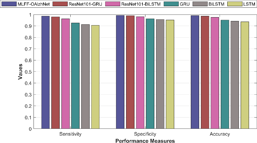
Figure 3: Sensitivity, Specificity, and accuracy

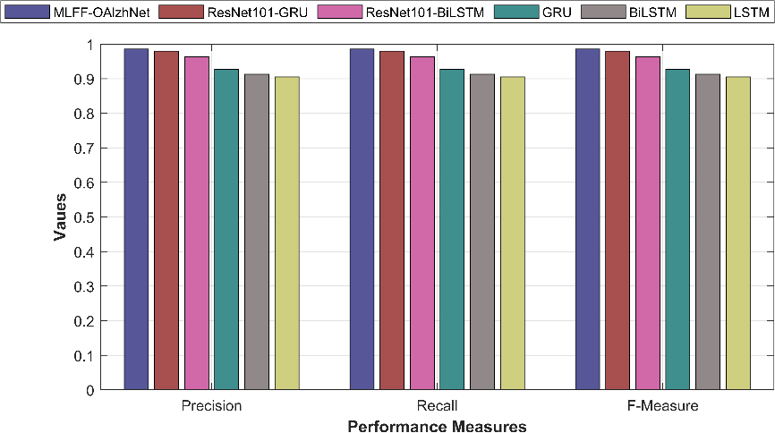
Figure 4: precision, recall, and F-measure

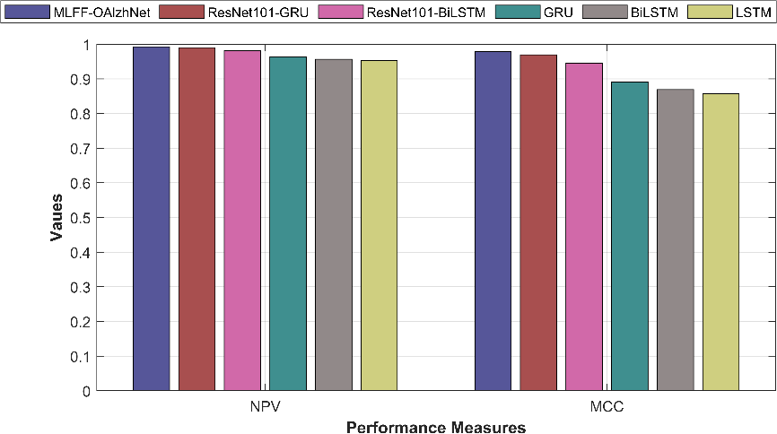
Figure 5: NPV and MCC

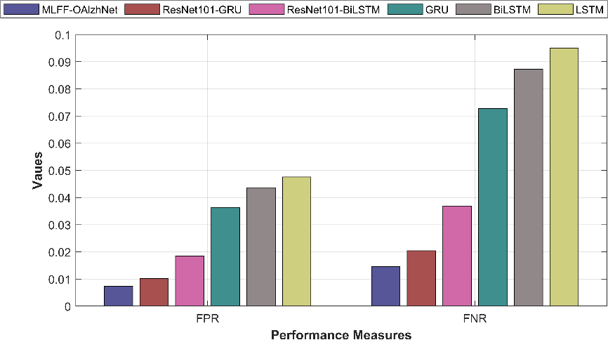
Figure 6: FPR and FNR

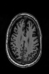
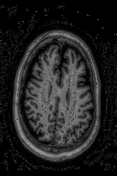
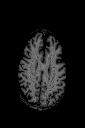
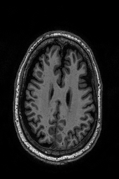
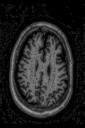
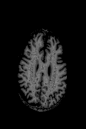
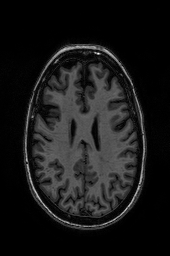
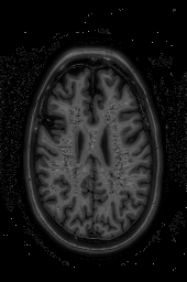
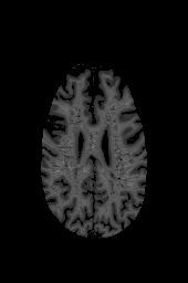
Figure 7: (a) original image (b) pre-processed image (c) classified image

Figure 7 illustrates the image processing pipeline: (a) shows the original image, (b) the pre-processed version, and (c) the classified result.

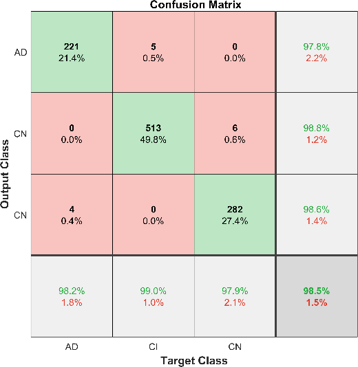
Figure 8: Confusion Matrix

(a)

(b)

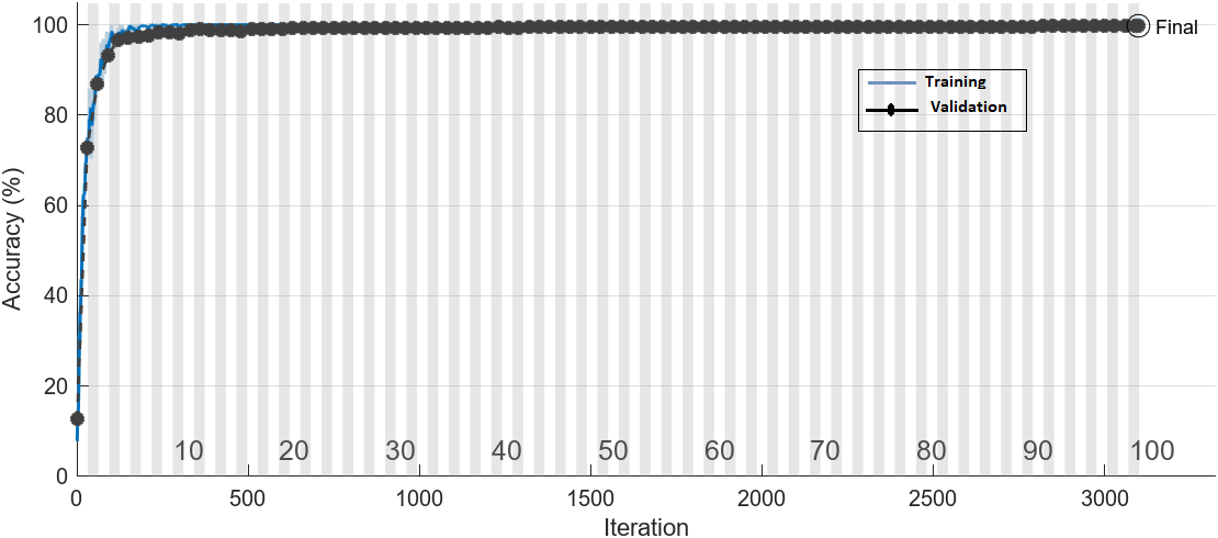
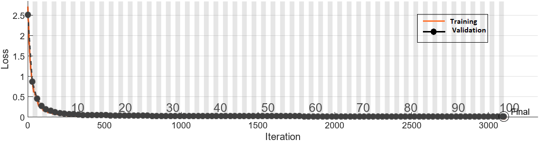
Figure 9: Validation (a) accuracy and (b) loss

The confusion matrix in Figure 8 shows the model’s correct and incorrect predictions. Figure 9 presents the validation accuracy and loss curves used to examine generalisation to unseen data.

Conclusion

In order to improve the classification and segmentation of MRI scans for AD, a novel metaheuristic-driven approach was developed in this study. The research framework comprised four key steps, beginning with data collection from an open-access online repository with a dataset encompassing four different AD classes. Modern methods were used to improve the MRI pictures, including local entropy-weighted histogram equalisation made possible by an AWDO algorithm. The implementation of guided filter-based picture denoising was also made possible because of the superior performance of the ASSO algorithm. With the last classification layer skipped, the core of this method used deep learning to extract spatial features using a ResNet152-based model. Otsu’s thresholding was incorporated into the segmentation process, which was then improved using the cutting-edge OBO method by combining elements of OOA and HBA to provide the ideal thresholding and extremely effective segmentation. The feature extraction phase was equally thorough; it included SIFT features, which were carefully concatenated with the ResNet152 features to enhance the feature representation, as well as GLCM, texture features (Mean, Variance, and entropy), edge features using the Canny edge detection method, and edge features. With DGRU being used for improved AD classification, this combination of multiple traits considerably strengthened the classification process.

References

Liu, J., Li, M., Luo, Y., Yang, S., Li, W. and Bi, Y., 2021. Alzheimer’s disease detection using depthwise separable convolutional neural networks. Computer Methods and Programs in Biomedicine, 203, p.106032.

Dogan, S., Baygin, M., Tasci, B., Loh, H.W., Barua, P.D., Tuncer, T., Tan, R.S. and Acharya, U.R., 2023. Primate brain pattern-based automated Alzheimer’s disease detection model using EEG signals. Cognitive Neurodynamics, 17(3), pp.647-659.

Amini, M., Pedram, M.M., Moradi, A., Jamshidi, M. and Ouchani, M., 2021. Single and combined neuroimaging techniques for Alzheimer’s disease detection. Computational Intelligence and Neuroscience, 2021.

Nawaz, H., Maqsood, M., Afzal, S., Aadil, F., Mehmood, I. and Rho, S., 2021. A deep feature-based real-time system for Alzheimer disease stage detection. Multimedia Tools and Applications, 80, pp.35789-35807.

El-Sappagh, S., Abuhmed, T., Islam, S.R. and Kwak, K.S., 2020. Multimodal multitask deep learning model for Alzheimer’s disease progression detection based on time series data. Neurocomputing, 412, pp.197-215.

Safi, M.S. and Safi, S.M.M., 2021. Early detection of Alzheimer’s disease from EEG signals using Hjorth parameters. Biomedical Signal Processing and Control, 65, p.102338.

Maqsood, M., Nazir, F., Khan, U., Aadil, F., Jamal, H., Mehmood, I. and Song, O.Y., 2019. Transfer learning assisted classification and detection of Alzheimer’s disease stages using 3D MRI scans. Sensors, 19(11), p.2645.

Janghel, R.R. and Rathore, Y.K., 2021. Deep convolution neural network based system for early diagnosis of Alzheimer’s disease. Irbm, 42(4), pp.258-267.

Mehmood, A., Maqsood, M., Bashir, M. and Shuyuan, Y., 2020. A deep Siamese convolution neural network for multi-class classification of Alzheimer disease. Brain sciences, 10(2), p.84.

Sathiyamoorthi, V., Ilavarasi, A.K., Murugeswari, K., Ahmed, S.T., Devi, B.A. and Kalipindi, M., 2021. A deep convolutional neural network based computer aided diagnosis system for the prediction of Alzheimer’s disease in MRI images. Measurement, 171, p.108838.

Li, W., Lin, X. and Chen, X., 2020. Detecting Alzheimer’s disease Based on 4D fMRI: An exploration under deep learning framework. Neurocomputing, 388, pp.280-287.

Ying, Y., Yang, T. and Zhou, H., 2023. Multimodal fusion for alzheimer’s disease recognition. Applied Intelligence, 53(12), pp.16029-16040.

Murugan, S., Venkatesan, C., Sumithra, M.G., Gao, X.Z., Elakkiya, B., Akila, M. and Manoharan, S., 2021. DEMNET: a deep learning model for early diagnosis of Alzheimer diseases and dementia from MR images. Ieee Access, 9, pp.90319-90329.

Shankar, K., Lakshmanaprabu, S.K., Khanna, A., Tanwar, S., Rodrigues, J.J. and Roy, N.R., 2019. Alzheimer detection using Group Grey Wolf Optimization based features with convolutional classifier. Computers & Electrical Engineering, 77, pp.230-243.

Ludwig, N., Fehlmann, T., Kern, F., Gogol, M., Maetzler, W., Deutscher, S., Gurlit, S., Schulte, C., Von Thaler, A.K., Deuschle, C. and Metzger, F., 2019. Machine learning to detect Alzheimer’s disease from circulating non-coding RNAs. Genomics, proteomics & bioinformatics, 17(4), pp.430-440.

Odusami, M., Maskeliūnas, R. and Damaševičius, R., 2022. An intelligent system for early recognition of Alzheimer’s disease using neuroimaging. Sensors, 22(3), p.740.

Puente-Castro, A., Fernandez-Blanco, E., Pazos, A. and Munteanu, C.R., 2020. Automatic assessment of Alzheimer’s disease diagnosis based on deep learning techniques. Computers in biology and medicine, 120, p.103764.

Talo, M., Yildirim, O., Baloglu, U.B., Aydin, G. and Acharya, U.R., 2019. Convolutional neural networks for multi-class brain disease detection using MRI images. Computerized Medical Imaging and Graphics, 78, p.101673.

Kruthika, K.R., Maheshappa, H.D. and Alzheimer’s Disease Neuroimaging Initiative, 2019. Multistage classifier-based approach for Alzheimer’s disease prediction and retrieval. Informatics in Medicine Unlocked, 14, pp.34-42.

Liu, L., Liu, S., Zhang, L., To, X.V., Nasrallah, F. and Chandra, S.S., 2023. Cascaded multi-modal mixing transformers for alzheimer’s disease classification with incomplete data. NeuroImage, 277, p.120267.

Mehmood, A., Maqsood, M., Bashir, M. and Shuyuan, Y., 2020. A deep Siamese convolution neural network for multi-class classification of Alzheimer disease. Brain sciences, 10(2), p.84.

AbdulAzeem, Y., Bahgat, W.M. and Badawy, M., 2021. A CNN based framework for classification of Alzheimer’s disease. Neural Computing and Applications, 33, pp.10415-10428.

Basheera, S. and Ram, M.S.S., 2020. A novel CNN based Alzheimer’s disease classification using hybrid enhanced ICA segmented gray matter of MRI. Computerized Medical Imaging and Graphics, 81, p.101713.

An, N., Ding, H., Yang, J., Au, R. and Ang, T.F., 2020. Deep ensemble learning for Alzheimer’s disease classification. Journal of biomedical informatics, 105, p.103411.

Fan, Z., Xu, F., Qi, X., Li, C. and Yao, L., 2020. Classification of Alzheimer’s disease based on brain MRI and machine learning. Neural Computing and Applications, 32, pp.1927-1936.

Dataset collected from: “https://www.kaggle.com/datasets/katalniraj/adni-extracted-axial” dated 10-04-2023.

Khan, M.H., Ulasyar, A., Khattak, A., Zad, H.S., Alsharef, M., Alahmadi, A.A. and Ullah, N., 2022. Optimal Sizing and Allocation of Distributed Generation in the Radial Power Distribution System Using Honey Badger Algorithm. Energies, 15(16), p.5891.

Dehghani, M. and Trojovský, P., 2023. Osprey optimization algorithm: A new bio-inspired metaheuristic algorithm for solving engineering optimization problems. Frontiers in Mechanical Engineering, 8, p.1126450.

Editorial Staff

Academic Master Education Team is a group of academic editors and subject specialists responsible for producing structured, research-backed essays across multiple disciplines. Each article is developed following Academic Master’s Editorial Policy and supported by credible academic references. The team ensures clarity, citation accuracy, and adherence to ethical academic writing standards

Content reviewed under Academic Master Editorial Policy.

• Editorial Staff

  Grid-Connected Solar PV Systems and Power Quality Review
• Editorial Staff

  Predicting Cardiovascular Diseases with PCA and Artificial Neural Networks
• Editorial Staff

  Maternal and Neonatal Outcomes Following Water Birth Systematic Review and Meta-Analysis
• Editorial Staff

  Electrospun Polymeric Nanofibers for Biomedical Applications