CA-DDGRU AlzNet for Alzheimer MRI Segmentation and Classification

ABSTRACT

Alzheimer’s disease is a heterogeneous, progressive, multifactorial neurodegenerative disease whose symptoms vary among patients. Early detection is therefore critical for both patient care and clinical research. The proposed deep learning-based model provides high performance in terms of segmentation and classification by executing cascaded feature learning. Therefore, cascaded deep learning is developed based on base model U-NET in which entropy enhanced Adaptive Batch Normalization, Gaussian enhanced Adaptive Batch Normalization, and dilated convolutions are newly introduced in the architecture. Non-demented, very mildly demented, mildly demented, and moderately demented are the four classes of the ADNI dataset considered in this research work. Compressive pooling layers, including Recurrent Kalman Filters and a Recurrent Median Filter, are introduced and connected to a Dense Gated Recurrent Unit (DGRU). The Cascaded U-Net with Dense GRU (CDGRU) provides highly efficient feature learning and classification performance. The proposed model is named as a Cascaded Dilated Dense-GRU based Alzheimer detection Network (CA-DDGRU: AlzNet).

The research emphasizes various performance metrics such as Accuracy, Precision, Recall, F1-Measure, Sensitivity, receiver operating characteristics (ROC), and confusion matrix to achieve high level segmentation and classification. Our proposed model shows an accuracy of 98% when compared with the various existing models like Support Vector Machine (SVM) of 87%, k-nearest neighbor (k-NN) of 65%, Decision Tree (DT) of 77%, Random Forest (RF) of 83%, Gradient Boosting (GB) of 85% and GaussianNB of 73% accuracy. An ADNI dataset of 6400 images is used for training and testing the proposed model. Existing models like VGG16, Siamese Network, MLP, CBLSTM+GAIN and CBLSTM+SMOTE show an accuracy of 95%, 92%, 89%, 82% and 82% respectively whereas our proposed Cascaded U-Net with Dense GRU outperforms the traditional methods with an accuracy of 98.1%.

Keywords: Alzheimer Disease (AD), cascaded feature learning, Machine Learning (ML), Magnetic Resonance Imaging (MRI), Dense Gated Recurrent Unit (DGRU).

Introduction

Alzheimer’s disease (AD) is a prevalent kind of dementia that is characterized by a decrease in memory and cognitive abilities. Preclinical, moderate cognitive impairment, and dementia are the three categories. While moderate cognitive impairment impairs language, reasoning, recollection adjustments, and judgment, preclinical dementia occurs in young adults under the age of 65. Huntington’s disease, Creutzfeldt-Jakob disease, Lewy body disease, vascular dementia, Parkinson’s disease, and Wernicke-Korsakoff syndrome are all caused by dementia [1].Alzheimer’s Disease (AD) is a major dementia-causing disease, causing memory loss, cognitive decline, and mood changes. It primarily affects the limbic system, with hippocampus and amygdala members suffering the most. Most patients go through a mild cognitive impairment stage before experiencing serious symptoms. Classification of AD using brain images can be improved using Artificial Neural Networks (ANN), which are inspired by the human brain’s structure. Deep Neural Networks (DNNs) use hidden layers to train models accurately [2]. Alzheimer’s disease is a neurological condition that progressively impairs behaviour, memory, and judgment. Research emphasizes early detection and treatment. Brain metabolic activity can be found using functional magnetic resonance imaging (fMRI), a new neuroimaging technique. In computer vision and medical image processing, deep convolutional networks in artificial intelligence are used to research AD [3]. Alzheimer’s disease and related dementia disorders are a significant global disability and cost, with an estimated global cost of $2 trillion by 2030. Researchers are working on non-invasive early detection methods and treatments. Current research methodologies, including speech and language processing, are suitable for early detection of cognitive impairment and AD. Deep learning, CNN, LSTM, and CNN-LSTM are used to detect AD from conversational transcripts [4]. Alzheimer’s disease is a gradual form of cognitive decline and brain degeneration. An MRI can show brain shrinkage and structure, which helps with AD diagnosis. For diagnosis, deep belief networks trained on specific brain areas are employed. Convolutional neural networks have been used in computer vision and image categorization [5]. Alzheimer’s disease (AD), which accounts for 70% of cases globally and causes dementia and cognitive decline, is a neurological illness. It starts 20 years before to the onset of symptoms and causes memory loss and linguistic difficulties. With the Alzheimer’s Disease Neuroimage Initiative dataset enhancing Deep Learning models for AD detection, computer-aided diagnosis is becoming more and more important [6]. Alzheimer’s disease costs $818 billion, affects 50 million people, and is the 7th largest cause of mortality in the world. The main dementia under investigation in this study is Alzheimer’s disease. A deep convolutional recurrent neural network and a bidirectional recurrent neural network are used by an Alzheimer Disease Assessment Engine to categorize dementia. Automatic generating also utilizes the Feature Sequence Generator [7]. Dementia, a neurological disorder causing memory loss and cognitive decline, is a common symptom in elderly individuals. Diagnosing AD is challenging due to the complexity of brain tissue structures and the difficulty in visualizing changes caused by AD. Therefore, proper classification techniques using brain images are necessary [8]. Without effective preventative methods, the Alzheimer’s Association anticipated that the number of AD cases will increase to nearly 100 million by 2050. Early diagnosis and early treatment techniques have been the subject of AD research. For early illness identification and the distinction between mild cognitively impaired patients and non-converter individuals, accurate diagnosis and prognosis are essential. Effective therapy and intervention depend on precise diagnosis and prognosis [9]. Research using deep neural networks (DNNs) to simulate acoustics and achieve better recognition outcomes than Gaussian Mixed Models has considerably enhanced voice modeling. This makes new voice recognition applications possible, such as speech-based AD detection. Acoustic embeddings can be extracted using automated speech recognition (ASR) algorithms to improve automatic analysis. The phonetic segmentation and labeling of input signals by ASR models based on convolutional deep neural networks can provide acoustic parameters including speech rate, pause rate, and hesitation rate [10]. For the diagnosis and treatment of many diseases, including brain cancer, cardiovascular disorders, liver cancer, and pulmonary disease, medical image segmentation is essential. The capacity of deep learning (DL) models to automatically learn important data attributes has led to their effectiveness in segmenting medical pictures. Medical image segmentation research has employed convolutional neural networks (CNN), with the U-Net model being the most well-known. Encoder-decoder architectures, however, are limited in their ability to generalize to various tasks and acquire multi-scale characteristics. A generalized encoder-decoder model for medical image segmentation dubbed the dense dilated inception network (DDI-Net) has been suggested to address these issues [11]. In biomedical applications, deep learning techniques, such as convolutional neural networks (CNNs) and recurrent neural networks, are used to handle complex, high-dimensional data, recognize images, model sequences, and detect DNA base modifications and predict protein-RNA binding [12]. The use of functional magnetic resonance imaging (fMRI) can provide light on the anomalies in brain activity that occur in psychotic illnesses. For the diagnosis of mental disorders using fMRI, deep learning techniques like functional connectivity and deep neural networks have gained popularity. The performance of classification has been enhanced using a hybrid framework integrating DNN and C-RNN [13]. Alzheimer’s is a prevalent disease that affects people 65 and older and causes significant memory loss, behavioural problems, and trouble doing daily tasks. A deep learning method is being used in a study to categorize older people’s fundamental daily activities (ADLs). The system represents the subject’s pose utilizing sequential pose data from CCTV cameras, human pose estimate, and LSTM architectures for classification [14]. Brain tumors are large, either benign or malignant growths that push on the meninges and create uneven growth, limiting the brain’s capacity to control the body. The World Health Organization’s tumor classification and grading system is used to forecast outcomes, standardize communication, and plan treatment for the more than 120 different forms of brain tumors that exist globally. According to the cell type and grade used for classification, primary tumors develop from cells of the brain’s tissue, whereas metastatic cancers spread there. Brain anatomy may be studied using medical imaging techniques including magnetic resonance imaging (MRI), computed tomography (CT), single-photon emission computed tomography (SPECT), and positron emission tomography (PET), but MRI is less radiation-insensitive [15]. These databases are commonly used in studies to classify Alzheimer and identify it early. Therefore, the proposed CC-DDGRU:AlzNet is emerged by executing a detailed literature review which is given in the following section.

Literature Review

Machine learning and deep learning are used in research to categorize and evaluate patients, predict treatment outcomes, and assess risks. Researchers used deep learning and machine learning methods to classify neurodegenerative disorders caused by AD and their stages through imaging-based detection. As a result of Deep Learning, it can preprocess the biomarkers itself and extract the features, as well as develop a model to identify AD and its stages.

Wang et. al., in 2020 have introduced the dense adaptive cascade forest (daForest). Compared to the original cascade forest, the deep forest ensemble and dense adaptive cascade forest (daForest) perform better. They began by employing the SAMME.R boosting method, which ensures improvement as the number of layers rises. This model then connects each layer to the one below it in a feed-forward manner, improving the model’s ability to fend off performance degradation. Finally, a layer for hyper-parameter optimisation is added before the initial classification layer, which reduces the amount of time needed to set up and determine the best hyper-parameters for this model [16]. Kundaram et. al., in 2020 have proposed a deep convolutional neural network (DCNN) for Alzheimer’s disease classification using magnetic resonance imaging (MRI) samples. High-level features can be learned using deep learning techniques from a dataset. The disease is categorised using this method as either Alzheimer’s disease (AD), mild cognitive impairment (MCI), or normal control (NC). To model DCNN, Spyder software from the Anaconda bundle with the Keras library and Tensorflow backend on GPU is utilised. When compared to other studies, the output classification result of the experiments using the ADNI dataset. We can extend this methodology to predict for more disease classification stages thanks to our approach [17]. Mehmood et. al., in 2020 have developed a Siamese convolutional neural network (SCNN) model inspired by VGG-16 (also called Oxford Net) to classify dementia stages. In modern clinical research, techniques based on deep convolutional neural networks (CNN) and machine learning are employed to detect AD using highly discriminative characteristics extracted from MRI images. They extended the sparse and unbalanced data utilising augmentation techniques, and trials were carried out using the open access series of imaging studies (OASIS) dataset. In terms of performance, efficiency, and accuracy, this model performed better than the most advanced models [18].

Various MR image sequences offer more detailed information and are crucial for clinical diagnosis and lesion analysis of brain illnesses. These supervised learning-based techniques need labelled datasets, which are frequently challenging to acquire. Mao et. al., in in 2022 have proposed an unsupervised learning-based generative adversarial network with adaptive normalization (AN-GAN) for synthesizing T2-weighted MR images from rapidly scanned diffusion-weighted imaging (DWI) MR images. Better feature maps are produced as a result of the image fusion operation, which also directs GAN training. Their method of synthesising T2 pictures provides superior perceptual quality and detail to other cutting-edge methods, according to experimental data. The lack of robustness of these models against varying artifacts impedes their use in medical applications where safety is critical [19]. Researchers observe a significant performance disparity because of model unfairness and put lots of effort to tradeoff between model performance and fairness. To tackle these issues, Xu, Zikang, et al, in 2023 have proposed FairAdaBN by making batch normalization adaptive to sensitive attributes. In order to evaluate the trade-off between model performance and fairness a new metric, named Fairness-Accuracy Trade-off Efficiency (FATE) is also included. Experiments on two dermatological datasets show that the proposed method outperforms other methods on fairness criteria and FATE [20].

He, Yefei, et al., 2023 have introduced a data-free quantization method for compressing neural networks to low bit-width without using the original training data. Adaptive batch normalization (ABN) is a technique introduced in the paper that addresses the quantization error caused by changes in the distribution of data during the process of model quantization. It updates the batch normalization layer adaptively to mitigate the impact of quantization on model performance. The proposed data-free quantization method, incorporating ABN, achieves significant improvements in accuracy compared to existing state-of-the-art methods [21].

Shamrat, FM Javed Mehedi, et.al, in 2023 have applied the CLAHE image enhancement method in ADNI database’s MRI scan dataset of 60000 image data on the 6 classes. This model is used to design the AlzheimerNet using RMSprop optimizer at a learning rate 0.00001 to achieve the highest test accuracy of 98.67%. The five pre-trained models and the proposed fine-tuned model were compared in terms of various performance matrices to demonstrate whether the AlzheimerNet model is in fact performing better in classifying and detecting the six classes. The model is able to classify individuals into the five phases of Alzheimer’s disease namely: MCI, EMCI, LMCI, SMC, AD, and overall, six classes, including NC. The performance of five different CNN models, VGG16, ResNet50, MobileNetV2, AlexNet, and InceptionV3 is compared to AlzheimerNet to determine the proposed model’s efficiency in performance. In this experiment hyperparameters are used based on ablation study. Parameters like accuracy, recall, precision, f1-score, etc. are computed from the confusion matrix and used to evaluate the models’ efficiency. Grad-CAM is designed to provide a visual representation. The suggested model outperforms the traditional methods for classifying Alzheimer’s disease stages from brain MRI, as measured by a two-tailed Wilcoxon signed-rank test, with a significance of < 0.05 [22].

The analysis of patient data obtained from electronic health records is not well suited for typical machine learning techniques like PCA. Merkelbach et. al., in 2023 have suggested a novel approach that directly involves in training a gated recurrent unit (GRU) autoencoder on health record data to address these problems. A recurrent neural network (RNN) architecture known as a GRU is used to analyze time series data, such as EHRs. By learning a low-dimensional feature space that encapsulates the patterns and dynamics of the patient data across time, it is intended to handle the temporal irregularity of the data. The GRU model makes it possible to identify discrete subgroups or classes of illness patterns in patients in the intensive care unit, opening the door to future improvements in personalized medication [23].

Segmenting medical images offers crucial hints for identifying disorders. Accurately separating long, narrow, and small organs from human bodies is quite difficult. Yuan, Feiniu, et al, in 2023 have suggested a Multiple Gated Boosting Network using Gated Recurrent Units (GRU) to address these issues. By including update and reset gates, GRU, which are frequently employed in image processing, are created to handle the difficulty of collecting long-term relationships in sequential data. By allowing the network to choose keep or reject input at each time step, these gates aid in the regulation of information flow inside the network, enhancing the network’s capacity to model complicated relationships and identify key features in medical image segmentation tasks [24]. Bakkouri, Ibtissam, et al, in 2019 have proposed a novel a Gated Recurrent Fusion Unit based Alzheimer’s Disease Recognition on sMRI based on 3D Multi-Scale CNN Features. Multiscale features are extracted via 3D Convolutional Neural Network and they are given as input to Gated Recurrent Units. It is designed to improve the performance of the system by incorporating gated recurrent units (GRU) for processing the extracted multi-scale features. The experimental results demonstrate that the proposed CAD system, with the inclusion of the GRFU, achieves state-of-the-art performance compared to existing methods, showing potential for enhancing recognition and classification strategies in clinical applications [25].

From our study, Ensemble models can enhance the representational ability of individual models and achieve better performance on prediction and generalization. On the other hand, processing large volume of data leads to ignoring critical data attributes, which has an impact on precision in decision making, whereas reducing data would result in performance degradation. A densely gated recurrent model can be used to adaptively select and fuse more effective information from multilevel features. Therefore, for more precise Alzheimer segmentation and classification, we proposed in this research a mixture of well-selected d GRU integrated with cascaded feature learning using multiple batch normalization process in U-Net model.

By considering various literature, the CA-DDGRU:AlzNet is developed by showing drastic improvement in U-Net and GRU based base models. The following shows the contribution of the proposed model.

Therefore, a CA-DDGRU: AlzNet model is developed based on Modified U-Net based segmentation and Dense GRU based classification. The following shows the contribution of the proposed model.

The U-Net based segmentation model is improved by introducing a novel Adaptive Batch Normalization in terms of

Entropy based Feature Extraction

Gaussian Mixer Model based Feature Extraction

In order to reduce the dimensionality of feature learning, two novel RNN based compressive feature learning strategy is adopted such as

Recursive Kalman Filter

Recursive Median Filter

The 2-level Dilated Convolution based feature learning strategy is adopted.

Phase 1: 1×1, 3×3, and 5×5

Phase 2: 1×1, 7×7, and 9×9

All these are applied on U-Net model for segmentation, and the classification Densely connected GRU is introduced.

Proposed Methodology

Data Collection and Preprocessing

The dataset is collected from the open-source reliable dataset (https://www.kaggle.com/datasets/tourist55/alzheimers-dataset-4-class-of-images). Preprocessing techniques are imperative for enhancing the quality of the dataset as raw data is typically contaminated with numerous noises that affects the segmenation performance especially the accuracy. It involves several steps such as noise removal through Gaussian filtering for image quality enhancement. The 2-D Gaussian distribution function employed by the proposed system’s Gaussian filter for a pixel (i, j) is provided as,

G_ij=d((1)/(2πσ²)e^{(-(i2+j2))/(2σ2)})=M (1)

Standard deviation, σ=√((∑_i=1ⁿ((d-μ)²))/(N)) (2)

Mean μ=(∑_i=1ⁿ(d_i))/(N) (3)

Where G represents the Gaussian, M represents the Input (i/p) data, σ denotes the standard deviation, N denotes the total number of elements. Then the preprocessed image is transferred into the CA-DDGRU: AlzNet for segmentation and classification

Modified U-Net based Segmentation

The proposed CA-DDGRU:AlzNet model is developed for obtaining a highly efficient segmentation and classification of Alzheimer’s disease. The overall flow of the proposed model is shown in Figure 1.

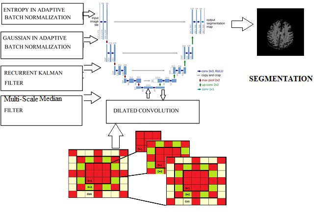
Figure 1: Overall Figure of the Proposed Model

Background Model

The U-Net is a type of convolutional network that possesses a modified U-shaped structure. It is typically used in the field of biomedical image segmentation, primarily thanks to its remarkable performance in the ImageNet dataset. The U-Net framework includes a fully convolutional network, accompanied by either a de-convolutional network or an encoder. These components are responsible for feature extraction and image contraction, while a decoder is employed for image expansion and segmentation. A remarkable advantage of the U-Net is its ability to accomplish the desired tasks with a reduced number of training images, resulting in extremely precise segmentation results. It consists of 3 sections (i) a down-sampling or encoding section (ii) up-sampling or decoding section (iii) bottle neck section.

Four contractions, or encoding blocks, make up the encoding portion. Each block’s input contains two convolutional layers, a kernel size of (3×3), a Relu activation function, a stride of 1, and the “he_normal” kernel initializer approach. The padding is ”same” and is followed by the dropout layer and max-pooling layer with the kernel (2×2), where the number of feature mappings doubles at each block. Four expansion blocks make up the up-sampling or decoding; each block has de-convolutional layers with kernel sizes of (2×2), (2×2) and padding of “same.” Following this are two convolutional layers using the same Relu activation function as in the encoding path. The stride is 1, the kernel initializer technique is “he_normal,” and the padding is “same.” The dropout layer then comes after it. The four convolution layers of the contraction or encoding blocks have (16, 32, 64, 128) output filters. Two convolutional layers with filter counts equal to 256 and a dropout layer make up the bottleneck region. The amount of feature maps produced by concatenating de-convolutional feature maps with feature maps from the encoding path is decreased by the two convolutional layers. For the output layer’s binary segmentation procedure, we employ a convolutional layer with a kernel of 1×1 and a sigmoid activation function.

In the Proposed modified UNET framework, we have presented a novel adaptive batch normalization technique that is rooted in the principles of entropy and Gaussian-based feature extraction. In addition to that,

Cascaded Feature Learning U-Net based Segmentation

The proposed Cascaded U-Net based Segmentation model includes five phases such as Entropy enhanced feature extraction, GMM enhanced Feature extraction, Recurrent Kalman Filters, Recurrent Median Filter, and Dilated Convolutional. Some techniques have been integrated with the traditional U-Net to enhance the performance of the overall model. The entropy and gaussian mixture model-based feature extraction techniques significantly improve the feature learning performance of the U-Net by understanding the modulations and the underlying structures present in the input data. The dilated convolutional in the U-Net brings several advantages like no loss of coverage and effectiveness more than the traditional convolutional layer. On the contrary, the utilization of Recurrent Kalman Filters and recurrent median filters facilitates the attainment of compressive features, whereby the parameters of the Kalman Filters and Median Filters are recurrently acquired through the Recurrent Neural Network (RNN). This facilitates the acquisition of enhanced feature acquisition, particularly in the context of feature space with a high number of dimensions, all while making efficient use of limited memory resources.

Dilated Convolutional Layer

The proposed Cascaded dilated U-Net model introduced a novel multi-level feature extraction framework built upon the principle of Dilated Convolutional layer, Recursive Kalman Filter, Recursive Median Filter, Entropy and Gaussian based Adaptive Batch Normalization. This approach significantly improves the performance of the proposed model. A 2-D convolutional can be defined as eq. (4):

y(o,p)=∑_i=1^o(∑_j=1^p(x(o+R×i, p+R×j)D(i,j))) (4)

The result of dilated convolution using the inputs x(o,p)and a filter D(i, j) with length and width of O and P, respectively, is y(o,p). The rate of dilation is the parameter R. Dilated convolution expands the receptive field without adding more parameters or computation (for example, adding more convolutional layers might increase receptive fields but add more operations). A small-size kernel with a k×k filter is enlarged to k+(k-1)(R-1)with a dilated stride R in dilated convolution. A dilated convolution becomes a regular convolution if R= 1. The expanded convolutional layer has implemented 1×1, 3×3, and 5×5 (ms1k, ms2k, and ms3k) kernels where Entropy based Adaptive Batch Normalization is employed with each kernel and combined (MS1=ms1k+ms2k+ms3k). In addition to the dilated Convolution improves the feature learning by executing the dilation with each filter. Therefore, the proposed model has the different filter size but a different dilation rate. Consequently, the suggested model possesses 3×3 filter with the dilation rates such as 1, 2, 3, 4, 8, 16, 32, 64, and 128. As similar to 3×3 filter, the same dilation rates can be added to 5×5 filters. Therefore, the filters get learned more feature from the input image. The use of dilation rates with larger filters can be beneficial in some cases. In addition to that, this can be helpful for tasks that require the CNN to see a large area of the input image, including semantic segmentation. The following Figure shows the illustration of (a)3×3, and (b) 5×5, filter based dilated convolution. The Following Figure 2. shows the dilation of the proposed model.

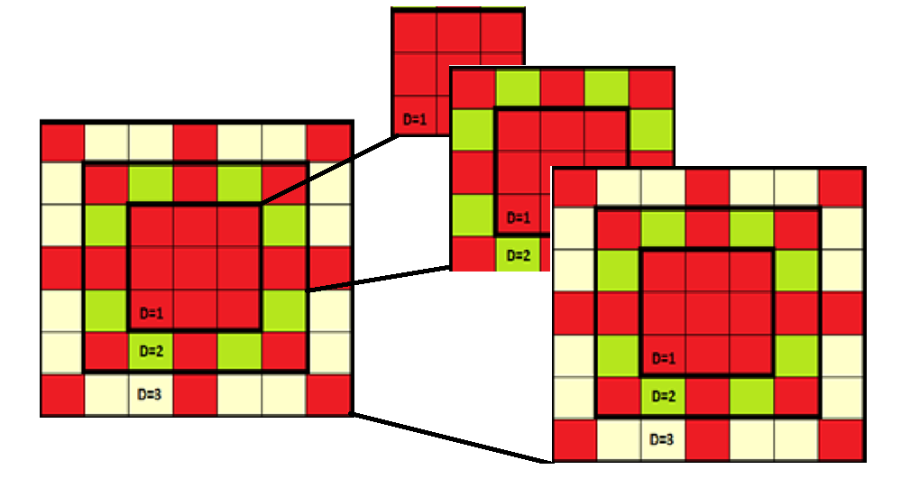
Figure 2: Dilation of 3×3 kernel

Finally, the concatenation of the 1×1, 3×3 and 5×5 are provided better results; therefore, the M₁sk₂(r_n), and M₁sk₃(r_n) and maintained into the D_msk1(Dilated Multi-Scale Kernel) as eq. (5).

D_msk1=∑_i=0ⁿ(M₁sk₁(r_n))+∑_i=0ⁿ(M₁sk₂(r_n)) (5)

Similarly, the dilation is applied on second level filters such as 1×1, 7×7, and 9×9. In which, the dilation is applied on each filter separately and then the filters are concatenated similar to the previous steps. Here, M₂sk₂(r_n) and M₂sk₃(r_n) are represented as the 7×7, and 9×9. These filters are concatenated as similar to D_msk1. The mathematical derivation of the step is shown below.

D_msk2=∑_i=0ⁿ(M₂sk₂(r_n))+∑_i=0ⁿ(M₂sk₃(r_n)) (6)

Then the final output of the D_msk1, and D_msk2 are concatenated (D_N) and its mathematical derivation as eq. (6).

D_N=D_msk1+D_msk2 (7)

Then the final feature vectors are fed into the subsequent layer.

Recurrent Kalman Filter

The Recurrent Kalman Filter (RKF) receives the D_N feature vector as input, which contains high-level features. Subsequently, the RKF performs recursive learning by integrating the advantages of RNN and KF. In the RKF, the initial process is conducted by considering the typical functioning of KF in decoding the brain’s Alzheimer region. The RKF has two models such as transition model and an observation model, with their respective mathematical representations provided as eq. (8).

x_i=Ax_i-1+w (8)

z_i=Hx_i+v (9)

Where, z_i is the where z_i is the D_N feature vector in the ith (i ∈ [t – l + 1, t]) time step and x_i denotes the variation in brain movement. A is the state transition matrix, H is the measurement transformation matrix, w and v are the state and measurement uncertainties drawn from Gaussian distributions N(0, Q) and N(0, R). With these parameters determined, KF utilizes an iterative feedback loop with a prediction step and an update step to fuse two models. In the prediction step, the mean and covariance of the current state are estimated by using eq.10 and eq.(12).

x_î= Ax_i-1 (10)

p_î= Ap_i-1A+Q (11)

where x_î is the prior state estimate for the ith time step and p_î denotes the prior state covariance matrix. In the update step, the Kalman gain k_î is calculated by using eq.(12).

k_î= p_î H^T(Hp_îH+R)^-1 (12)

Based on k_î and the observed measurement z_i, the mean and covariance of the posterior state estimate, i.e. x_i and p_i, can be updated as eq. (13) and eq.(14)

x_i=x_î+k_i(z_i-Hx_î) (13)

p_i= (I-k_îH) p_î (14)

I is the identity matrix, In conventional KF, the parameters A, H, Q, and R are constant matrices that must be manually created under generalizations that may be arbitrary and unrefined for many real-world applications. To assess the linear relationship between the anticipated temporal changes and obtain characteristics from the Alzheimer’s image, the transition model and observation model of KF are helpful. Similarly, the LSTM model is utilized for capturing the non-linear dynamics between the input and output based on dataset. The mathematical derivation of the proposed LSTM is derived as eq.(15).

[i_i=δ[W_i[S_i-1, Z_i]+b_i]] ; [m_i=δ[W_m[S_i-1, Z_i]+b_m]] ; [[o_i=δ[W_o[S_i-1, Z_i]+b_o]] ; [c_i=i_i⊙tanh[W_c[S_i-1, Z_i]+b_c]+m_i⊙c_i-1] ; [[s_i=i_i⊙tanh(C_i)] ; [y_i=W_yS_i+b_y]]] (16)

At time-step i, s_i represents the hidden state, c_i is the activation vector, i_i is the input gate, m_i is the forget gate, o_i is the output gate, δ is the logistic sigmoid function, W is the matrix of gates and layers, b is the bias vector, and ⊙ is the scalar product. For future forecasts, model training will end the starting state. LSTM-KF follows the KF computational network in eq. (17)-(7), but focuses on learning A, H, Q, and R from data using multiple LSTM modules. The transition model uses LSTM modules to generate A_iand Q_i from x_i-1

A_is_i^A=LSTM_A( x_i-1, s_i-1^A) (17)

Q_is_i^Q=LSTM_Q( x_i-1, s_i-1^Q) (18)

A_i, R_i,Q_i and R_i are input into KF’s prediction and update steps to compute x_i-1 and P_i-1 LSTM-KF exhibits dynamic changes in both transition/observation and covariance matrices over time. K̂_i in eq. (19) represents the intermediate gain, and an additional LSTM module is used to get the ultimate gain K_i:

K_i,S_i^K=LSTM_K(K_î,S_i-1^K) (19)

Multi-Scale Median Filter

On the other hand, the Multi-Scale Median Filter (MS-MF) operates in a manner comparable to the Recursive Median Filter (RMF). The RMF utilizes a median filter to substitute the pixel value with the median of the grey levels within the pixel’s vicinity. The computation of the median incorporates the original value of the pixel. Median filters are widely utilized due to their exceptional ability to reduce specific forms of random noise, while causing far less blurring compared to linear smoothing filters of comparable dimensions. The computation of the median includes the initial value of the pixel. Median filters (M_f) are widely utilized due to their exceptional noise reduction capabilities for specific forms of random noise. Compared to linear smoothing filters of comparable size, median filters offer much reduced blurring. The M_f is derived by using eq. (20)

M_f=f̂(x,y)=[median] ; [(s,t)∈S_xy]{g(s,t)} (20)

The M_f is then applied with the multi-scale filters in order to enhance the feature learning performance. The mathematical derivation of the MS-MF is derived by using eq. (21) and eq. (22).

M_msk1=∑_i=0ⁿ(M₁sk₁(M_f))+∑_i=0ⁿ(M₁sk₂(M_f)) (21)

Where the values of the Multi-Scale Median Filter (MS-MF), enhances the feature learning performance. Similarly, the values obtained from the median filter is given into the second level multi-scale filter. The following mathematical derivation shows the second level multi-kernel filters.

M_msk2=∑_i=0ⁿ(M₂sk₁(M_f))+∑_i=0ⁿ(M₂sk₂(M_f)) (22)

The combination of the M_msk1 and the M_msk2 are fused together to obtain highly efficient feature vectors (MSMF_N) which is shown in eq. (23).

MSMF_N=M_msk1+M_msk2 (23)

Adaptive Batch Normalization

The original purpose of the Batch Normalization (BN) layer was to address the internal covariate shifting issue, which is a frequent issue when training a very deep neural network. Prior to learning a common slope and bias for each mini-batch, it first standardizes each feature in a mini-batch. Formally, given the input to a BN layer A∈R^s×d where s denotes the batch size, and d is the feature dimension, BN layer transforms a feature i ∈ {1 . . . d} into,

X_î= (X_i-E[A_i])/(√(var[A_i])), Y_i= δ_iX_î+α_i, (24)

where X_i and Y_i are the input/output scalars of one neuron response in one data sample; A_i denotes the ith column of the input data; and δ_i and α_i are parameters to be learned. This transformation ensures that each layer’s input distribution is maintained consistently across several mini-batches. In order to improve the performance of the batch normalization, Tsallis entropy based adaptive batch normalization is introduced.

Tsallis entropy based Batch Normalization

The Tsallis entropy T based features of the input image are applied on a Batch Normalization using the eq. (25) and (26).

s_q(p)=(1)/(q-1)(1-∑_x(p^q(x))) (25)

y_n= s_q(p) (26)

In this case p denotes the probability distribution of interest, q is a real parameter. In the limit as q 1. The feature extraction can be done using the segmented o/p and the Tsallis-Entropy o/p. The s_q(p) is having the entropy features which are applied to Batch Normalization as eq. (27).

X_î= (X_i-E[A_i])/(√(var[A_i])) +r(y_i+y_n) (27)

Where, r is the random variable [0-1] that prevents the premature convergence and the y_i and y_n are iteratively updated with adaptive batch normalization.

Similarly, GMM based features are also applied with the adaptive batch normalization, which helps to learn more effectively than the tradition batch normalization.

Gaussian mixture model (GMM)

GMM-based features exhibit promising accuracy as a classifier for separating target regions from ghost/clutter regions. According to GMM, a parametric probability density function, it is a weighted sum of T component Gaussian densities.

P((y)/(β))= ∑_i=1^T(m_i(y\γ_i,∑_i( ))) (28)

Where y represented the n dimensional continuous valued data vector, m_i the mixture weight, and G the component of Gaussian densities.

Each component density was controlled by the n variate gaussian function according to

G(y\γ_i,∑_i( ))= (1)/((2π)^n/2|∑_i( )|^1/2) exp {-(1)/(2) (y- γ_i)^v(∑_i( ))^-1(y- γ_i)}, (29)

Where γ_i is the average of a vector, v is the transpose, and ∑_i( )is the covariance matrix.

The mean vectors, covariance matrices, and mixture weights from all component densities were used to parameterize the entire Gaussian mixture model. These parameters can be expressed according to

σ={m_i,γ_i,∑_i( )} (30)

The variance (c_i) of components was represented by the diagonal of the covariance matrix ∑_i( )we extracted then a feature vector r_gmm from three components of GMM according to

r_gmm={m₁…m_3,γ₁…γ₃, c₁…c₃} (31)

Where, m, γ and c are the weight, average and variance of GMM components

The r_gmm is applied on Batch Normalization for improving the performance of U-Net.

X_ĝ= (X_i-E[A_i])/(√(var[A_i])) +r(y_i+r_gmm) (32)

Where, X_ĝis adaptive batch normalization that obtained by using GMM.

With all these advanced features, the modified U-Net executes the better segmentation outcome. The Table I shows the sample I/p and segmentation o/p obtained from the segmentation phase of the CA-DDGRU:AlzNet.

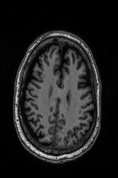
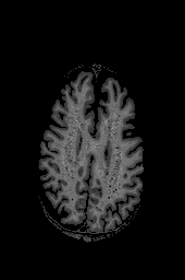
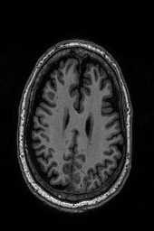
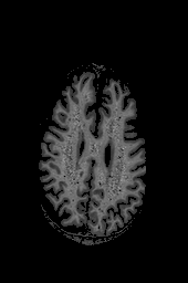
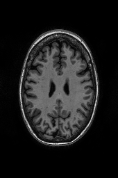
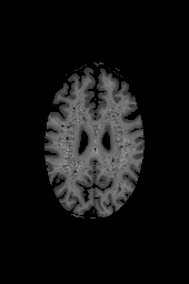
In the Table I, the segmentation o/p obtained from the CA-DDGRU:ALzNet is provided where I/P shows three different inputs and the O/P shows three segmented image from the given I/P.

Dense GRU Based Classification

The GRU model is trained on feature obtained from the previous layer. Specifically, the GRU model uses the past information captured by its cell value and current observation to predict the next observation. Assume a training set {x_i∈ R^d, i=1, …., N} are collected under a moving window approach can be applied, with the window length being n, n ≪N. Here, h_i∈ R^d_h, denotes the hidden state of the first layer at the ith time, h_i^‘ ϵ R^d_h‘ denotes
the hidden state of the second layer, h_i^” ϵ R_h^d” denotes the hidden state of the third layer and x̂_n+1 ∈ R^d is the predicted value. The hidden state h_i of the first layer becomes the input to the second layer of GRU model. Take the first window as an example, the structure of a three-layer GRU is shown in Figure 3.

The final output is then obtained using the dense layer as eq. (33).

x̂_n+1 = W^‘h_n^‘+ b^‘ (33)

Here x̂_n+1 is the prediction of x at the n + 1th time instance, W^‘ is the weight matrix of the dense layer, b^‘ is the bias term. A GRU model with more layers can also be used, for the sake of simplicity, however three-layer GRU is considered here.

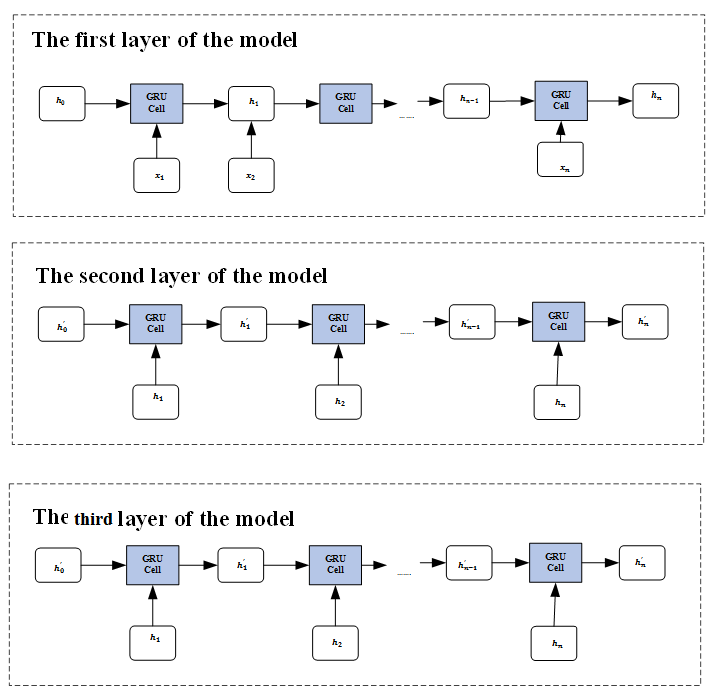
Here, h_i∈ R^d_h, denotes the hidden state of the first layer at the ith time, h_i^‘ ϵ R^d_h‘ denotes
the hidden state of the second layer, h_i^” ϵ R_h^d” denotes the hidden state of the third layer and x̂_n+1 ∈ R^d is the predicted value. The hidden state h_i of the first layer becomes the input to the second layer of GRU model. Then the second layer of GRU output is fed into the third GRU where the final output is then forward into the dense layer as follows.

x̂_n+1 = W^‘h_n^‘+ b^‘

Here x̂_n+1 is the prediction of x at the n + 1th time instance, W^‘ is the weight matrix of the dense
layer, b^‘ is the bias term. A GRU model with more layers can also be used, for the sake of simplicity,
however three-layer GRU is considered here.

The model parameters can be trained based on the N – n + 1 windows. Once the model parameters are estimated, estimation of model output x̂_n+1 can be predicted from the past n samples. A series of residuals can be obtained as e_i=|x̂_i – x_i|, i=n+1,….,N. The dense layer executes the classification by utilizing the loss function as follows.

Figure 3: Architecture of the Dense GRU

The model parameters can be trained based on the N – n + 1 windows. Once the model parameters are estimated, estimation of model output x̂_n+1 can be predicted from the past n samples. A series of residuals can be obtained as e_i=|x̂_i – x_i|, i=n+1,….,N. The self-attention mechanism at the end of each GRU layer to provide varying degrees of attention to the content of different relevance. The dot product, the cosine similarity, and the splicing similarity are used in the attention mechanism. The scaled dot product is utilized to assess the similarity between two points in this paper. The mathematical derivation of the attention mechanism is shown in eq. (34).

sim(Q,K)=(Q×K^T)/(√(d_k)) (34)

where Q and K are represented as query and key respectively. d_k is the length of the K vector. The eq.(35) is the mathematical derivation of the self-attention.

X̃=∑_j=1ⁿ(w_ij×softmax(sim(Q,K)×V)) (35)

WhereX̃ o/p, w_ij weight coefficient, V represents the value. These parameters are identical in this work. The SA is incorporated with the GRU provides better classification performance then in subsequent step, where dense layer is adopted for classicisation.

Result and discussion

On MATLAB 2023 platform with a 24GB GPU, the proposed model has undergone testing. The suggested model is trained using a batch size of 16, a parameter of 50 epochs, and an initial learning rate of 0.001. With our Proposed model and by imitating a small amount of human visual reasoning, interpretable image classification predictions are made. In brain imaging, Cascaded U-Net with Dense GRU based segmentation techniques will play a crucial role in the diagnosis and classification of Alzheimer’s disease (AD). Our results on AD classification have more accuracy than those of their black-box competitors while also offering clear model justifications. On comparing the proposed model with other models including Gaussian NB(Naive_bayes) (GNB), k-nearest neighbor (k-NN), Decision Tree (DT), Random Forest (RF), and k-NN the results are tabulated. With the testing dataset our proposed model of Cascaded U-Net with Dense GRU exhibit some encouraging results in terms of overall accuracy, precision, recall, F1-measure, sensitivity, receiver operating characteristics (ROC), and confusion matrix values.

Overall Analysis

The Cascaded U-Net with Dense GRU approach has low false positive (FP) and false negative (FN) rates of 40 and 45, respectively and the greatest true positives (TP) of 3783.3 and true negatives (TN) of 6028.8. The accuracy of this model is 0.98 and it also has the highest sensitivity (0.9647) and specificity (0.9682). Table II compares the accuracy (A), precision (P), recall (R), f1-measure (f1), sensitivity (S) of different machine learning algorithms.

Table II: Comparative analysis of performance metrics with various ML algorithm

In comparison to the k-nearest neighbor model, our suggested model has a maximum accuracy percentage of 0.98 and a least accuracy % of 0.65. Figure 4 compares the proposed model’s accuracy percentage to that of other current models.

Figure 4 Overall accuracy comparison with various ML algorithms

Our CA-DDGRU: AlzNet model has the highest precision percentage of 0.96, whereas Support Vector Machine, k-nearest neighbor, and Decision Tree models have the lowest precision percentages of 0.54. In a similar vein, our suggested model shows a maximum recall percentage of 0.97 while Support Vector Machine and Random Forest model shows a least remember percentage of 0.59. Additionally, our suggested model has an f-measure maximum value of 0.96 while the k-nearest neighbor model has an f-measure minimum value of 0.49. The comparison of the CA-DDGRU: AlzNet model with various different machine learning algorithms is represented graphically in Figure 5.

Figure 5 Overall performance comparison of different metrics using various ML algorithms

Performance analysis of CA-DDGRU:AlzNet – ADNI dataset

We consider the MRI modality for this research work because it has more imaging flexibility, excellent tissue contrast, is free of ionizing radiation, and can provide useful information on human brain anatomy. Other available modalities include Positron Emission Tomography (PET), genotype sequencing results, etc. For researching different metrics for the performance analysis in AD classification, we used ADNI datasets. In terms of accuracy, precision, recall, and F-measure the suggested model obviously surpasses all the previous models.

Table III: Comparative analysis of performance metrics – ADNI dataset

A visual representation of the performance metrics comparison analysis for the ADNI dataset can be found in Figure 6. The x-axis lists various models that were assessed, and the y-axis displays the value of each measure. According to the graph, our proposed CDGRU model has the greatest values, scoring 0.98, 0.96, 0.97, and 0.96 respectively.

Figure 6: Comparative analysis of performance metrics – ADNI dataset

Classification based performance analysis of proposed model

After the necessary pre-processing is completed, the CA-DDGRU:AlzNet algorithm technique is used to train with four classes of the Kaggle dataset in order to conduct severity classification in the early diagnosis of Alzheimer’s disease. Non-demented, very mildly demented, mildly demented, and moderately demented are the 4 classes present in the dataset. The collection consists of 6400 photos in total. 1280 of these photos are used for testing, while the remaining 5120 are used to train the model. Whereas 64 images are classified as very demented, 896 images are classified as mildly demented, 2240 images are classified as very mildly demented, and 3200 images are classified as non-demented. Figure 7 shows the proposed model’s total accuracy percentage after training, which resulted in an accuracy of 94.1%.

Table IV: Classification based comparative analysis of performance metrics

Figure 7: Classification based overall accuracy percentage of CA-DDGRU:AlzNet models

Conclusion

Alzheimer’s disease is an inimical form of dementia that affects brain cells which inversely affect the memory, thinking capacity, and even affect the ability to perform most basic tasks. This Proposed model that intends to improve the accuracy of recognizing and categorizing AD, which relies on structural MRI. The proposed model CA-DDGRU:AlzNet in which entropy enhanced Adaptive Batch Normalization, Gaussian enhanced Adaptive Batch Normalization, and dilated convolutions are newly introduced along with Compressive pooling layers such as Recurrent Kalman Filters, and Recurrent Median Filter and fed into Dense Gated Recurrent Unit (DGRU).This proposed Cascaded U-Net with Dense GRU model extract discriminative features from the ADNI dataset’s raw input data. These input data are augmented and normalized to manipulate the class imbalance with the input data. The dataset comprises four classes namely mild demented, moderate demented, non-demented, very mildly demented and our proposed model shows a high rate of accuracy (98.1%) in comparison with existing models tabulated in Table IV. Accuracy, Precision, Recall, F1-Measure, Sensitivity, ROC, and confusion matrix are the major performance metrics used in this research work.

The effective detection of AD is accomplished using a variety of techniques, including DTI, PET, FLAIR, and genetic sequencing results. These biomarkers enable the investigation of numerous classes and the employment of numerous strategies to recognize the various stages of AD. As future work, a hybrid model of MRI with other dataset can be used in segmentation and classification of AD.

References

Chamarajan, Gowthami, and Y. Charishma. “Alzheimer’s Disease: A Survey.” International Journal of Artificial Intelligence 8, no. 1 (2021): 33-39.

Hazarika, Ruhul Amin, Debdatta Kandar, and Arnab Kumar Maji. “An experimental analysis of different deep learning based models for Alzheimer’s disease classification using brain magnetic resonance images.” Journal of King Saud University-Computer and Information Sciences 34, no. 10 (2022): 8576-8598.

Li, Wei, Xuefeng Lin, and Xi Chen. “Detecting Alzheimer’s disease Based on 4D fMRI: An exploration under deep learning framework.” Neurocomputing 388 (2020): 280-287.

Mahajan, Pranav, and Veeky Baths. “Acoustic and language based deep learning approaches for Alzheimer’s dementia detection from spontaneous speech.” Frontiers in Aging Neuroscience 13 (2021): 623607.

Li, Fan, Manhua Liu, and Alzheimer’s Disease Neuroimaging Initiative. “A hybrid convolutional and recurrent neural network for hippocampus analysis in Alzheimer’s disease.” Journal of neuroscience methods 323 (2019): 108-118.

Khojaste-Sarakhsi, M., Seyedhamidreza Shahabi Haghighi, SMT Fatemi Ghomi, and Elena Marchiori. “Deep learning for Alzheimer’s disease diagnosis: A survey.” Artificial Intelligence in Medicine 130 (2022): 102332.

Chien, Yi-Wei, Sheng-Yi Hong, Wen-Ting Cheah, Li-Hung Yao, Yu-Ling Chang, and Li-Chen Fu. “An automatic assessment system for Alzheimer’s disease based on speech using feature sequence generator and recurrent neural network.” Scientific Reports 9, no. 1 (2019): 19597.

Hazarika, Ruhul Amin, Ajith Abraham, Samarendra Nath Sur, Arnab Kumar Maji, and Debdatta Kandar. “Different techniques for Alzheimer’s disease classification using brain images: a study.” International Journal of Multimedia Information Retrieval 10, no. 4 (2021): 199-218.

Aghili, Maryamossadat. “Deep Learning for Multiclass Classification, Predictive Modeling and Segmentation of Disease Prone Regions in Alzheimer’s Disease.” (2021).

Yang, Qin, Xin Li, Xinyun Ding, Feiyang Xu, and Zhenhua Ling. “Deep learning-based speech analysis for Alzheimer’s disease detection: A literature review.” Alzheimer’s Research & Therapy 14, no. 1 (2022): 1-16.

Bala, Surayya Ado, and Shri Kant. “Dense dilated inception network for medical image segmentation.” international Journal of Advanced Computer Science and Applications 11, no. 11 (2020).

Wang, Jade Xiaoqing, Yimei Li, Xintong Li, and Zhao-Hua Lu. “Alzheimer’s Disease Classification Through Imaging Genetic Data With IGnet.” Frontiers in Neuroscience 16 (2022): 846638.

Zhao, Min, Weizheng Yan, Na Luo, Dongmei Zhi, Zening Fu, Yuhui Du, Shan Yu, Tianzi Jiang, Vince D. Calhoun, and Jing Sui. “An attention-based hybrid deep learning framework integrating brain connectivity and activity of resting-state functional MRI data.” Medical image analysis 78 (2022): 102413.

Hong, Lim Chin, Connie Tee, and Michael Kah Ong Goh. “Activities of Daily Living Recognition Using Deep Learning Approaches.” Journal of Logistics, Informatics and Service Science 9, no. 4 (2022): 129-148.

Taşcı, Burak. “Attention Deep Feature Extraction from Brain MRIs in Explainable Mode: DGXAINet.” Diagnostics 13, no. 5 (2023): 859.

Wang, Haiyang, et al. “Dense adaptive cascade forest: a self-adaptive deep ensemble for classification problems.” Soft Computing 24.4 (2020): 2955-2968.

Kundaram, Swathi S., and Ketki C. Pathak. “Deep learning-based Alzheimer disease detection.” Proceedings of the Fourth International Conference on Microelectronics, Computing and Communication Systems: MCCS 2019. Springer Singapore, 2021.

Mehmood, Atif, et al. “A deep Siamese convolution neural network for multi-class classification of Alzheimer disease.” Brain sciences 10.2 (2020): 84.

Mao, Yanyan, et al. “Generative adversarial networks with adaptive normalization for synthesizing T2-weighted magnetic resonance images from diffusion-weighted images.” Frontiers in Neuroscience 16 (2022): 1058487.

Xu, Zikang, et al. “FairAdaBN: Mitigating unfairness with adaptive batch normalization and its application to dermatological disease classification.” arXiv preprint arXiv:2303.08325 (2023).

He, Yefei, et al. “Data-Free Quantization with Accurate Activation Clipping and Adaptive Batch Normalization.” Neural Processing Letters (2023): 1-14.

Shamrat, FM Javed Mehedi, et al. “AlzheimerNet: An effective deep learning based proposition for alzheimer’s disease stages classification from functional brain changes in magnetic resonance images.” IEEE Access 11 (2023): 16376-16395.

Merkelbach, Kilian, et al. “Novel architecture for gated recurrent unit autoencoder trained on time series from electronic health records enables detection of ICU patient subgroups.” Scientific reports 13.1 (2023): 4053.

Yuan, Feiniu, et al. “A multiple gated boosting network for multi‐organ medical image segmentation.” IET Image Processing (2023).

Bakkouri, Ibtissam, et al. “Recognition of Alzheimer’s disease on sMRI based on 3D multi-scale CNN features and a gated recurrent fusion unit.” 2019 international conference on content-based multimedia indexing (CBMI). IEEE, 2019.

Editorial Staff

Academic Master Education Team is a group of academic editors and subject specialists responsible for producing structured, research-backed essays across multiple disciplines. Each article is developed following Academic Master’s Editorial Policy and supported by credible academic references. The team ensures clarity, citation accuracy, and adherence to ethical academic writing standards

Content reviewed under Academic Master Editorial Policy.

• Editorial Staff

  Grid-Connected Solar PV Systems and Power Quality Review
• Editorial Staff

  Predicting Cardiovascular Diseases with PCA and Artificial Neural Networks
• Editorial Staff

  Maternal and Neonatal Outcomes Following Water Birth Systematic Review and Meta-Analysis
• Editorial Staff

  Electrospun Polymeric Nanofibers for Biomedical Applications