
Abstract
autonomous vehicles (AV) or self-driving cars got more and more into the focus of the automotive industry. Object detection and tracking is essential in AV. To overcome the challenges of various methods used for the object detection and tracking in autonomous vehicles, a method called a three-fold-deep-learning and optimized deep semantic segmentation network (O-DSNN) is proposed. In this method, pre-processing is done using the Image resizing, Image normalization, Colour space conversion, Noise reduction and Contrast adjustment techniques followed by the segmentation using the optimized Deep Semantic Segmentation Network (O-DSSN). Using the segmented data, the next step called feature extraction is done. Color-based features, Texture-based features, Shape-based features and Histogram-based features are utilized by which the features are extracted. Finally, classification is done using the three-fold-deep-learning model and Hybrid optimization algorithm called Gazelle Customized Spider Monkey Optimization (GC-SMO) is utilized to optimize model parameters. The suggested approach has an accuracy of %, specificity of %, sensitivity of %, Precision of %, F measure of %. Thus, from the results, it is seen that our suggested approach performs better in comparison to the other existing methods.
Keywords: Autonomous vehicles, DSNN, GOA, SMO
Introduction
Autonomous vehicles (AV), also known as self-driving cars, have gained more and more attention in recent years from both the automotive sector and emerging mobility companies. Commercial cars currently come equipped with a variety of automation features, including adaptive cruise control, assisted or automated parking, and even highway pilots. They need a very accurate system of environmental awareness that can handle any imaginable circumstance in order to achieve the maximum level of automation. Furthermore, real-world scenarios necessitate real-time performance. Modern automobiles come with a variety of sensors, including radar, cameras, ultrasonics, and Lidar (light detection and ranging). Relevant security and reliability can be attained via redundancy and sensor fusion [1]. There are 4 basic divisions that can be made for the autonomous vehicle system. Several various sensors put on the vehicle are used to sense the environment. These are pieces of hardware that collect environmental data. The perception block, whose components turn sensor data into information with meaning, processes the information from the sensors. The output from the perception block is used by the planning subsystem for both short- and long-range path planning as well as behaviour planning. Control module transmits control commands to the vehicle and makes sure it follows the path specified by the planning subsystem [2]. Based on their stationarity across the training and test sets, obstacles can be divided into two types. 1. Stationary Objects (SO): Scene elements like roadways and residences that are completely stationary. 2. Non-Stationary Static Objects (NSSO): Static objects that changed position or vanished in the course of the mapping and re-localization processes [3]. Interconnected optical and sensory reactions to the environment are a part of autonomous vehicle awareness systems, which necessitate complicated real-time decision-making for human safety [4]. Based on the sensory inputs they use, traditional autonomous vehicle techniques can be divided into three categories: dense point clouds from range sensors, vision sensors, and a fusion of range and vision sensors [5].
One of the most significant and difficult areas of computer vision is object recognition and tracking, which has found extensive use in a variety of industries including health monitoring, autonomous vehicles, anomaly detection, and more. The efficiency of object detectors and trackers has significantly increased thanks to the rapid advancement of deep learning (DL) networks and GPU computing capability. DL networks or image processing methods can both be used for object detection. Object tracking comes after object detection. The purpose of object tracking is to identify and connect an observed object's trajectory [6]. There are two different categories inside the object detection framework. Both conventional and DL -based detectors are used. The sub-parts of DL detectors include two-stage detectors and one-stage detectors, for example. Various techniques are available to detect these autonomous cars [7,8]. For DL to be used in practical settings, such as autonomous driving, it must be able to detect objects regardless of image distortions or environmental factors. Stylizing the training images is a straightforward data augmentation technique that significantly improves sensitivity for corruption types, severity, and data [9]. Autonomous driving requires 3D multi-object tracking. Its objective is to calculate throughout time the positions, orientations, and sizes of all the objects in the environment. It promises to pinpoint the motions of many moving item categories, including vehicles, bicycles, and pedestrians. Planning to enable autonomous driving is aided by this [10]. The fundamental building block of the perception stack is 3D object detection, particularly for the purposes of path planning, motion prediction, and collision avoidance. [11]
The potential for autonomous driving to drastically alter urban environments and save many lives is enormous. The identification and monitoring of agents in the environment around the vehicle are essential components of safe navigation. A modern self-driving vehicle uses a variety of sensors and advanced detection and tracking algorithms to accomplish this. These methods rely more and more on machine learning (ML), necessitating benchmark datasets [12]. The data gathered by touch sensors can be interpreted using artificial intelligence (AI) methods. For these aims, many ML techniques are employed [13]. The perception systems in autonomous vehicles must be precise, reliable, and real-time. In computer vision, DL has been quite successful. Given a lot of data, a deep neural network is an effective tool for learning hierarchical feature representations [14]. The majority of computer models for generic and domain-specific object detection are based on DL. In most object detectors, these computational models serve as the backbone architecture, and they are employed to carry out a number of operations such feature extraction from an input image, segmentation, classification, and object localisation, among others. Autonomous vehicles perform better, are more efficient, and experience fewer accidents when appropriate technologies for object recognition and tracking are used [15]. The contribution of the work is as follows,
Using the dataset, pre-processing, segmentation, feature extraction and classification is done.
Hybrid optimization algorithm called Gazelle Customized Spider Monkey Optimization (GC-SMO) is utilized to optimize model parameters by which the performance will be improved.
The recommended method and existing methods are compared and the results are obtained based on the evaluation metrics.
Finally, the suggested method enhances the model by resulting higher accuracy.
The main section of the paper is as follows. The Section 2 explains about the Related Work, Section 3 explains the proposed part and Section 4 shows the Results and Discussions and finally Section 5 gives the Conclusion of the paper.
Related Work
Yaran Chen et.al [16] developed a unique Cartesian product-based multi-task combination strategy to simultaneously model object identification and distance prediction using multi-task learning (MTL). In addition, we mathematically demonstrate that, when the multi-task itself is not independent, the suggested Cartesian product-based combination method is superior to the linear multi-task combination technique typically utilised in MTL models. Systematic tests reveal that the suggested method consistently outperforms both the single-task and multi-task dangerous object detection approaches in terms of object detection and distance prediction.
Ze Liu et.al [17] discussion of to overcome the inherent limitations of a single sensor in bad weather, radar and camera information fusion sensing techniques are applied. Radar serves as the primary hardware in our fusion strategy, with cameras serving as the secondary hardware. In addition, the target sequence's observed values are matched using the Mahalanobis distance. Fusion of data using the joint probability function approach. Additionally, real sensor data from a vehicle was used to verify the algorithm's ability to perceive the environment in real-time. The test findings demonstrate that radar and video fusion algorithms outperform single sensor environmental perception in bad weather, dramatically lowering the rate of missed detection for autonomous vehicles. The environment perception system's resilience is increased by the fusion algorithm, which also gives autonomous cars' decision-making and control systems accurate environment perception data.
S.Murugan et.al [18] addresses the use of augmented reality head-up displays (AR-HUDs) powered by ML in autonomous vehicles. The suggested model has completed the processes of object detection and classification of the obtained HUD data. Based on the AR environment, determining the current state of the vehicle has been validated. Test and validation procedures are an essential part of the development cycle. In this paper, lab and real-world testing and verification for ARHUD and autonomous vehicles are done using ML and deep neural networks. The simulation's findings are based on the information acquired by the application of human and machine interface (HMI) to identify items and categorise things in motion. The simulation results obtained are accuracy of 98%, precision 94%, recall 92.3% and F-1 score 86%.
Desheng Xie et.al [19] proposed a system for autonomous vehicle obstacle identification and tracking based on three-dimensional light detection and ranging (LiDAR). The obstacle is clustered using the eight-neighbor cells clustering approach that has been proposed. By fusing the real-time kinematic data from the autonomous vehicle's inertial navigation system and global positioning system, static obstacle detection of multi-frame fusion is developed based on the clustering results. We also use the results of the static obstacle detection to look for moving obstacles that are present in the travelable region. The moving obstacle is then tracked steadily using an upgraded dynamic tracking point model and a Kalman filter, and its steady movement state is obtained at that point. Numerous tests on the autonomous car that we developed show that the approach has higher reliability.
Nayereh Zaghari et.al [20] explores how deep neural network techniques (LSV-DNN) are used to train self-driving cars based on actual driving behaviour. The goal of this study is to create a convolutional network for an autonomous vehicle's motion planning utilising behavioural cloning and a DL framework. Neural networks are powerful tools for categorising data, predicting new data, and modelling relationships between data. Neural networks can estimate steer angle and speed for autonomous driving as a result of using real data as input. In comparison to previous methods, this method has low FPR and FNR and great accuracy and speed.
S.Bhaggiaraj et.al [21] s claims that the field of autonomous vehicles has been revolutionised by AI integration of sophisticated models and algorithms. The current innovations face challenges due to modelling architecture's overly sophisticated, expensive, and difficult-to-understand state-of-the-art findings. The Automatic Land Vehicle in Neural Network (ALVINN), which is now used by self-driving vehicles using a naive approach, has a complex model architecture that makes it challenging to interpret. The performance and functionality of autonomous vehicles will therefore be enhanced and improved by a self-driving vehicle based on DL. to understand the input of probable safety problems. A good autonomous driving system should deliver precise results, be simple to use, and be affordable.
Aryan Mehra et.al [22] Image dehazing is essential to any vehicular motion and navigation work on the road or in the air. It was proposed as a concept to provide safe and smooth operations in frequent bad weather scenarios. This model makes use of ReViewNet, a dehazing technology that is quick, light, and reliable and is appropriate for autonomous cars. The network effectively removes haze from images taken by autonomous vehicle cameras using techniques including spatial feature pooling, quadruple color-cue, multi-look architecture, and multi-weighted loss. The proposed method is shown to be effective in different hazy weather circumstances for autonomous vehicle applications by qualitative investigation of the efficiency of the proposed model with particular use cases and visual responses on distinctive vehicular vision instances.
Anum Aleem et.al [23] a proposal for Target Classification of Marine Debris Using DL was proposed. They gave an explanation of the DL-based architecture used to identify and categorise maritime garbage. The Histogram Equalisation method and Median Filter are used to increase contrast and eliminate noise in photographs. Intense Forward-Looking Sonar Image (FLS) Marine Debris Dataset experiments are run. There are ten different categories of debris in this dataset. The suggested technique categorises the debris into ten kinds in addition to detecting it. Faster-RCNN with transfer learning of ResNet-50 architecture is utilised to address the problem of data scarcity. One of the widely used object detection designs, Faster-RCNN, simultaneously employs a detector and a Regional Proposal Network (RPN). This results in better performance.
Problem Statement
Object detection and tracking (ODT) in autonomous vehicles uses various DL methods. The methods in use may be complicated and the performance was around 95%. Autonomous vehicles perform better, are more efficient, and experience fewer accidents when appropriate technologies for object recognition and tracking are used. To improve the performance of the ODT in AV, a method called three-fold-deep-learning and optimized deep semantic segmentation network (O-DSNN) is suggested which uses a optimization called Gazelle Customized Spider Monkey Optimization by which the results are classified with higher accuracy.
Proposed System
A method called a three-fold-deep-learning and optimized deep semantic segmentation network (O-DSNN) is proposed. In this method, pre-processing is done using the Image resizing, Image normalization, Colour space conversion, Noise reduction and Contrast adjustment techniques followed by the segmentation using the optimized Deep Semantic Segmentation Network (O-DSSN). Using this segmented data, feature extraction is done using Colour-based features, Texture-based features, Shape-based features and Histogram-based features by which the features are extracted. Finally, classification is done using the three-fold-deep-learning model and Hybrid optimization algorithm called Gazelle Customized Spider Monkey Optimization (GC-SMO) is utilized to optimize model parameters. Fig 1shows the Block illustration of proposed methodology.
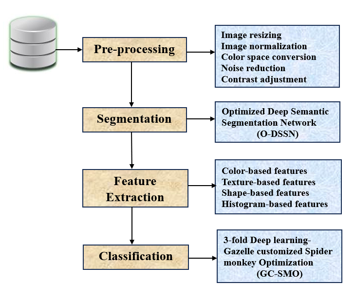
Fig 1: Block illustration of proposed methodology
3.1. Pre-processing
The initial step is the Pre-processing. The data pre-processing is a significant step for transforming the raw dataset into a most suitable format. The pre-processing involved in conversion, image resize, noise removing enhances the quality of the images. The main benefit of an efficient preprocessing step is improved segmentation results, which lead to superior classification accuracy. The dataset may contain some redundant information and noise signal. Consider a dataset as , where xdata, ycorresponding class, f features, N number of instances.
3.1.1. Image resizing
It is possible to assure consistent input dimensions for the model and lower the amount of computing by resizing the photographs to a standard size. To ascertain how different sizes affect the recognition process, the photographs included in the investigation are resized in various scales. The optimum image size must be carefully considered because different image sizes transmit different information. Resizing an image has the effect of reducing its data size, which reduces processing time. Different image sizes are produced by the resize scale, which randomly changes between 0.1 and 0.9 values. An image can be resized to change its aspect ratio, make it smaller, or make it larger. Bicubic interpolation and bilinear interpolation are two common image scaling methods. The image resizing of data is given in (1),
(1)
3.1.2. Image normalization
Data normalisation is one of the pre-processing techniques in which the data is scaled or altered to ensure that each feature contributes equally. The image's pixel values can be brought closer to a particular range, such as [0, 1] or [-1, 1], by normalising them. The Min-Max Normalisation (MMN) approach is used to achieve this; it linearly scales the unnormalized data to a predetermined lower and upper bound. This enhances model stability and convergence during training. It is given in (2),
(2)
Where and represents minimum and maximum values of the feature, and lower and upper bounds to rescale the data.
3.1.3. Colour space conversion
Images can be represented differently by converting them to different colour spaces, such as RGB (Red, Green, Blue), HSV (Hue, Saturation, Value), or grayscale. These representations may be more suited for particular activities or highlight certain elements.
3.1.3.1. Converting RGB to HSV
RGB are co-related to the colour luminance (intensity). We cannot separate color information from luminance. HSV used to separate image luminance from color information.
(3)
(4)
(5)
3.1.3.2. Converting RGB to grayscale
RGB image to grayscale is usually based on luminance. It converts RGB images to grayscale by eliminating the H and S information while retaining the luminance. It is represented as,
(6)
The coefficients 0.299, 0.587, and 0.114 are commonly used to approximate the luminance.
3.1.4. Noise reduction
Clarity of significant features will be enhanced by using the denoising technique known as Gaussian blur to minimise noise in the photos. It is a low pass filter. Every pixel in an image has calculated for it. When there is Gaussian noise in the image, the filter is extremely helpful. It's stated as,
(7)
Standard deviation, (8)
Mean (9)
Where denotes distances to the X and Y axis, denotes standard deviation
3.1.5. Contrast adjustment
The visibility of details and overall image quality can both be improved by increasing the contrast of images using adaptive histogram equalisation (AHE). The image enhancement technique is among the most significant methods used in picture processing. It is essential to improve the image's visual appeal. The CLAHE is an expansion of the AHE. The CLAHE method was initially created as a way to transform poor contrast medical photographs into images of higher quality. The limitation of the contrast value is where CLAHE and AHE diverge. By cropping the histogram based on user-specified values known as clip limits, CLAHE restricts amplification. The clipping level determines how much noise in the histogram needs to be smoothed, therefore some contrast should be raised. In this instance, the histogram boundary will automatically adjust to the boundary level, and modifications will be made to raise the excess histogram limit in the image background area. A bell-shaped histogram is typically created using the distributed Rayleigh histogram border,
(10)
is the minimum pixel value, is the nonnegative real scalar, is the cumulative probability distribution.
3.2. Segmentation
The pre-processed data is used for segmentation. Utilising a new segmentation technique called the optimised Deep Semantic Segmentation Network (O-DSSN), it is utilised to recognise foreground items. To accomplish precise and effective object segmentation, O-DSSN combines the strength of DL architectures with semantic segmentation. Because semantic segmentation assigns each pixel in an image to a certain class, it is also known as pixel-level categorization. In order to grasp the content of an image, it is crucial to segment an image or classify pixels according to their local properties and texture features.
The process of assigning a class label to each pixel in a picture is known as semantic segmentation. Semantic segmentation has been utilised for many years in many different applications, including road segmentation for autonomous driving and medical image analysis. SegNet is used in this study to separate the objects from the photos. For problems involving semantic segmentation, SegNet is suggested in. In this design, feature maps for segmentation are produced using pairs of encoders and decoders. The output image must be the exact same size as the original image. The input and output of auto-encoders are identical, making them a specific case of encoder-decoder types. Fig 2 shows the SegNet Architecture
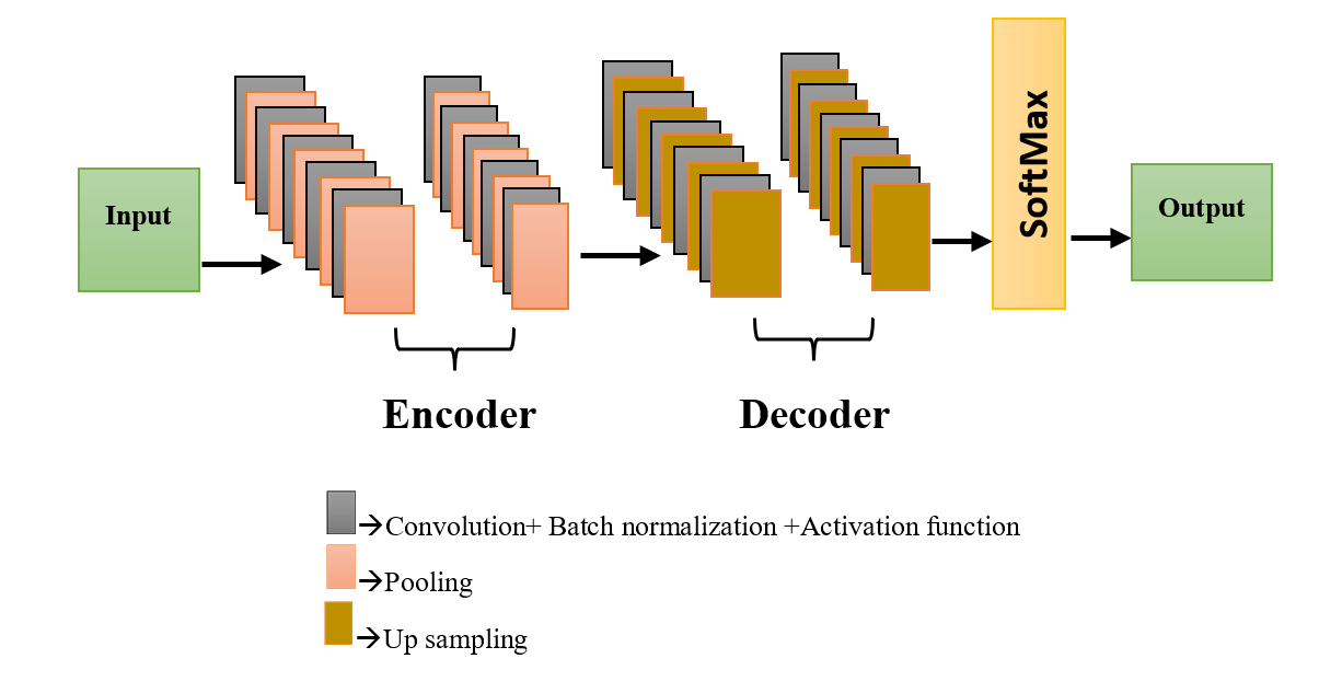
Fig 2: SegNet Architecture
3.2.1. Input layer
It is the initial layer which contains the input for the model by which the process is done.
3.2.2. Encoder network
It performs convolution with a filter bank to produce a set of feature maps. These are then batch normalized. Then an element-wise rectified linear non-linearity ReLU is applied. Following that, max-pooling with a 2 × 2 window and stride 2 (non-overlapping window) is performed and it is used to reduce the feature map size.
The convolution is given as,
(11)
Where , are the weights and bias, means input
The batch normalization (BN) is used to speed up the training. BN simply changes the mean and standard deviation of all the pixels in the feature maps in a convolution layer.
(12)
Where indicates Mean, indicates Standard deviation, are arbitrary constants
Activation function (ReLU) is used to decrease the non-linearity. It is given as,
(13)
Max Pooling is given as,
(14)
Finally, encoding is given as,
(15)
3.2.3. Decoder network
It uses the max-pooling indices from the appropriate encoder feature map(s) that it has memorised to up-sample the input feature map. Sparse feature maps are created in this step. Contrary to other network decoders, this one creates feature maps with the same number of channels and sizes as the encoder inputs. A trainable soft-max classifier receives the high dimensional feature representation at the output of the final decoder. Each pixel is classified separately by this soft-max. A K channel image of probabilities, where K is the number of classes, is the soft-max classifier's output. The class with the highest probability at each pixel corresponds to the segmentation that is expected. The decoding function is given as,
(16)
When normalising a neural network's output to a probability distribution over a projected output class, the SoftMax function is frequently employed as the final activation function. The probability will all add up to 1, and the range will be 0 to 1. It is given as,
(17)
3.2.4. Output layer
It is the final layer which contains the final result of the model. By using these results, the feature extraction will be done.
3.3. Feature Extraction
The feature extraction process is the next phase. It is done to obtain features that will be helpful in classification. From the segmented objects, various advanced feature extraction techniques are applied. In the proposed feature extraction step, handcrafted features are utilized to capture discriminative information from the segmented objects.
3.3.1. Colour-based features
The distribution or associations of the colour information in the segmented objects are captured by colour histograms. Due to its intuitive nature relative to other qualities and more significant information, ease of extraction from the image, and the way the histogram distributes collars using a series of boxes, colour is the most prevalent and commonly utilised feature. Even though the phrase "colour histogram" is more frequently associated with three-dimensional colour systems like RGB or HSV, it may be constructed for any type of colour space. The term intensity histogram may be used instead for monochromatic images. The histogram will be used as a model for the probability distribution of the intensity levels in the statistically based histogram features that we will take into consideration. These statistical features provide us with information about the characteristics of the intensity level distribution for the image. We define the first-order histogram probability, as:
(18)
Where represents total pixels in the image, represents total pixels at grey level g
3.3.2. Texture-based features
While texture features employ groups of pixels, colour features only use individual pixels. Each pixel in the feature maps has a Local Binary Pattern (LBP) calculated for it. It compares the information and then encodes the conclusions in binary form. A group of binary features that record specific local texture patterns are generated. It takes the segmented objects' surface features, such as patterns, edges, or edges, and extracts texture information from them. The LBP is a useful nonparametric operator for specifying localised picture properties. A central pixel'sgrey value is compared to the pixels of its eight neighbours to produce an ordered binary set that is defined as LBP. As a result, the LBP code is represented as an octet value in decimal form as,
(19)
Where is the grey value of the centre pixel , is the gray value of the pixels of its eight neighbors. LBP code has been proved to be invariant to any gray level transformation, and the local neighbourhood binary code remains unchanged after transformation
(20)
3.3.3. Shape-based features
The form features of the items are captured by Zernike moments. The features produced by applying a complicated set of Zernike polynomials to the input image are known as ZMs. Because it is rotationally invariant, the magnitude of these moments is used for recognition. By first calculating the radial polynomials and then projecting the input image onto the ZMs basis function, the ZMs features are calculated. The Zernike radial polynomials are given as,
(21)
is a non-negative integer is a nonzero integer;
The order of Zernike bias function is given as,
(22)
Where ,
The ZMs of order n and repetition m of a function f(x, y) are defined by,
(23)
Where is a complex conjugate of
3.3.4. Histogram based features
The appearance of the segmented item can be briefly represented using histograms of oriented gradients (HOG). By examining regional picture gradients within small regions, it accomplishes the gradient-based features. For shape and edge analysis, it generates features that capture information on gradient orientation and amplitude. This method counts instances of gradient orientation in a small section of a photograph. It is better than other edge descriptors since it computes the features using the gradient's magnitude and angle. The gradient of the image is calculated. The gradient is produced by adding the image's magnitude and angle. The gradient must be determined using a grayscale image. Each pixel's and are calculated, using,
(24)
(25)
Where f are rows, g are columns, is an image
Once and is calculated, and of a pixel is using the equations shown below to determine the value.
Magnitude (26)
Orientation, (27)
A pixel whose direction is near to orientation may be allocated another orientation because there are few directions. To get over this issue, every single cell is given two close-crypts, and depending on how the pixel gradient is oriented from two near-directional directions, a little portion of the gradient's size μ decreases linearly. The histogram channels are evenly spread over 0-1800 or 0-3600 depending on whether the gradient is unsigned or signed. As a result, there are four blocks covering each cell. One characteristic value b is obtained in each block when the four-cell histograms are combined.
(28)
is a minor positive constant to prevent division by zero in gradient-free units
To determine the HOG feature, all of the normalised blocks' features have been incorporated into a single vector.
(29)
Based on the above methods, the proper features are extracted,
Classification
This is the final step in the process which is very important because it classifies the result. The image classification accepts the given input images and produces final output. A new three-fold-deep-learning model that combines EfficientNet (E-N), Transfer Neural Network (TNN) and optimized ResNet (R-N) are employed to accurately classify objects into predefined classes. The proposed methodology incorporates advanced techniques for optimization and model training. Hybrid optimization algorithm called Gazelle Customized Spider Monkey Optimization (GC-SMO) is utilized to optimize model parameters and hyperparameters. Three-fold deep learning models are a popular choice for training and evaluating DL models because they are relatively simple to implement results in reduced training time and improved performance. To perform this three-fold-deep-learning model, initially split the dataset into three folds. Train an E-N on two folds of dataset then Train TNN on E-N model and finally Train R-N on TNN model. Determine the performance of each model on the last fold of the dataset and calculate the average performance of each model on the three test sets.
3.4.1. EfficientNet
The foundation of E-N Models is a straightforward and powerful compound scaling approach. Compound scaling uniformly scales each dimension with a predetermined fixed set of scaling coefficients as opposed to arbitrarily increasing width (w), depth (d), or resolution (r). The concept behind the compound scaling approach is to scale with a constant ratio in order to balance the dimensions of width, depth, and resolution. It is essential to balance network breadth, depth, and resolution during ConvNet scaling to achieve greater accuracy and efficiency.
Due to this, E-N models are able to perform better than earlier CNNs while using less FLOPs (floating point operations per second) and parameters. For instance, we can employ a model with a high value of if we need a network that is both accurate and effective. We can employ a model with a low value of if we require a compact and effective network. Efficiency and accuracy are improved with E-N models. It is explained how a compound coefficient is used in a compound scaling approach to evenly scale network breadth, depth, and resolution.
(30)
Where ;
,, are constants that can be determined by a small grid search, is a user-specified coefficient that controls how many more resources are available for model scaling.
3.4.2. Transfer Neural network:
Transfer neural network (TNN) is a neural network that can be used as a starting point for training a new neural network on a different task after being trained on a sizable batch of data for a particular task. To achieve this, the pre-trained network's early layer weights are frozen, and only the latter layer's weights are retrained for the current task. The overall loss function must be minimized in order to successfully train the TNN. The network will be encouraged to learn features that are advantageous for both the new task and the basic task as a result. The following formula can be used to calculate the loss function (L) for training a TNN:
(31)
Where indicates Loss on new task, indicates Loss on base task, indicates controls the weight given to the
3.4.3. ResNet
It is well known that ResNets can train extremely deep networks without running into the vanishing gradient issue. When training very deep neural networks, a phenomenon known as the vanishing gradient problem may arise in which the gradients of the loss function with respect to the network weights become very small. The network may find it challenging to learn as a result.
It employs the residual learning method to solve the vanishing gradient problem. The network can learn residual mappings—differences between a layer's input and output—through residual learning. As a result, even very deep networks find it simpler to learn the appropriate mapping. A stack of residual blocks is the standard building block for ResNets. A path is traced by two convolutional layers in each residual block. As a result, the network can learn identity mappings, which are input-neutral mappings. This improves the network's ability to learn residual mappings.
The identity path and skip path are the two basic paths that make up a residual block. The residual mapping, which is the difference between the desired output and the input to the block, is learned via the identity path. Bypassing the identity path, the shortcut path offers a direct connection for the input to flow through the block. The leftover block's output is provided as,
(32)
Where is Input, is residual mapping learned by the block
3.4.4. Gazelle Customized Spider Monkey Optimization (GC-SMO)
A population-based optimizer, the GOA. The GOA models a gazelle's capacity to live in a setting where a predator rules. One of the most popular prey species for predators is the gazelle. The mechanism of the GOA's functioning is characterised in two phases—exploration and exploitation—much like any other population-based algorithm. A random number is used to determine which step will be executed next. The exploitation phase is carried out if it is less than 0.5; else, the exploration phase is performed. The exploitation phase imitates the behaviour of gazelles while they quietly graze or when a predator is stalking them. The neighbourhood areas of the domain are effectively covered at this phase by the Brownian motion, which is characterised by uniform and controlled steps. In the exploitation stage,
(33)
Where ,are gazelles’ current and next position, represents matrix in which the top gazelle vector is replicated N time, is gazelles’ grazing speed, are random numbers for Brownian motion and random numbers in [0,1].
The exploration phase simulates the behavior of gazelles when they suddenly spot the predators and the behavior of the predators when they chase the gazelles. The population is divided into two equal groups. The first group represents gazelles, and the second group represents predators. The behavior of gazelles can be derived as follows:
(34)
Where is the maximum speed that gazelles can reach,is a vector of random numbers calculated using the Lévy distribution. regulates the predators’ movement, it varies at each iteration and is calculated
(35)
Where t is iteration, T is max iteration
The behavior of the predators can be formulated by,
(36)
In order to avoid trapping at local optima, the algorithm uses the effect of the predator success rates (PSR) to improve the quality of the solutions obtained as follows:
(37)
Where are random indices of two individuals in the population.
The research on Mongolian gazelles also claimed that even though the animals are not endangered, they have annual survivorship of 0.66, which translates to just 0.34 instances where predators are effective.
(38)
SMO is a meta-heuristic method that draws inspiration from spider monkeys' clever foraging behaviours. The fission-fusion social structure serves as the foundation for spider monkeys' foraging activities. The social organisation of a group where a female leader decides whether to separate or combine is what this algorithm's features are based on. A Spider Monkey (SM) represents a probable resolution in the SMO algorithm. There are six phases. These better balances exploitation and exploration while seeking the ideal spot while a predator is stalking them. At this stage, the Brownian motion, which is typified by uniform and controlled steps, effectively covers the domain's surrounding territories. The exploitation phase can be represented by the model below. The Local Leader (LL) phase is utilised to investigate the search region because during this phase, every group member updates their positions with significant dimensional disturbance. Better candidates have more opportunities to update their positions even though the GL phase encourages exploitation as it does in this phase. It is a preferable option among search-based optimisation techniques because of this characteristic. It also has a built-in mechanism to prevent stagnation. To determine whether the search process has stagnated, the local leader learning phase and global leader learning phase are used. Local leader and GL decision phases function in situations of stagnation (at the local or global level). While a judgement about fission or fusion is made in the GL decision phase, the local leader decision phase initiates additional exploration. As a result, it maintains the convergence pace while better balancing exploration and exploitation. Based on the fitness assessment in each phase, the optimum option is identified. Utilizing the above equation from SMO,
(39)
indicates dimension of Spider monkey, indicates position of Global leader in the jth dimension,indicates jth dimension of a randomly selected SM from the kth group such that , is a uniformly distributed random number in the range (0, 1). is a uniformly distributed random number in the range (-1, 1).
(40)
(41)
Where is a new position, is a current position represents Maximum Speed, is a best solution, is a random position in search space, are control coefficients when movement follows best solution, explores search space.
Finally, Kalman filter is used. It is used in situations where you have a system with uncertain or noisy measurements and you want to obtain the best estimate of the system's true state over time. It is widely used in applications such as navigation, tracking, control systems, and sensor fusion.
It has two states prediction and update state. The state prediction of standard Kalman filter is given as,
(42)
represents predicted state at time y, is an estimated sate at time y-1, is a state transition matrix is an observation matrix indicates system noise vector, is observation noise vector.
(43)
indicates prediction vector of at time y+1
The optimal estimation is given as,
(44)
(45)
Where is a Kalman gain at time y+1, is an actual observation of moving obstacle
at time y+1, prediction covariance matrix, means observation noise (with
(46)
Where is a state transition noise (with
Once the optimal estimation is done, update to ,
(47)
Where defines Identity matrix
Based on the above steps the Kalman filter will work and the stable tracking result of moving obstacle will be obtained. Finally, the results are classified in this stage.
Results and Discussion
Using the dataset taken, the results are evaluated using the performance metrices——. The results are computed in comparisons of the suggested and the existing methods—————- by implementing in a ——- platform.
4.1. Dataset Description:
————————–
4.2. Evaluation metrics:
The performance of the suggested and the existing approaches are done using the performance metrics called Accuracy, Sensitivity, Specificity, Precision, F measure, FNR, FPR and MCC.
4.2.1. Accuracy:
It is the proportion of true forecasts to all i/p Observations. It is calculated using the following formula,
(48)
4.2.2. Sensitivity
The fraction of real positives that are correctly identified is measured by sensitivity. It is given as,
(49)
4.2.3. Specificity
The percentage of real negatives that are accurately identified is measured by specificity. It is calculated using
(50)
4.2.4. Precision
How much of a model's positive predictions are actually right is determined by its precision, which is a performance indicator. In order to assess how well what you detect is actually present, precision is important. It is given as,
(51)
4.2.5. F measure
A general score for performance evaluation, the F1-score is a combination statistic that combines Precision and recall. It is given as,
(52)
Conclusion
To overcome the challenges of various methods used for the object detection and tracking in autonomous vehicles, a method called a three-fold-deep-learning and optimized deep semantic segmentation network (O-DSNN) is proposed. In this method, pre-processing is done using the Image resizing, Image normalization, Colour space conversion, Noise reduction and Contrast adjustment techniques followed by the segmentation using the optimized Deep Semantic Segmentation Network (O-DSSN). Using this segmented data, feature extraction is done using Color-based features, Texture-based features, Shape-based features and Histogram-based features by which the features are extracted. Finally, classification is done using the three-fold-deep-learning model and Hybrid optimization algorithm called Gazelle Customized Spider Monkey Optimization (GC-SMO) is utilized to optimize model parameters. The suggested approach has an accuracy of %, specificity of %, sensitivity of %, Precision of %, F measure of %. Thus, from the results, it is seen that our suggested approach performs better in comparison to the other existing methods.
References
[1] Simon, Martin, Karl Amende, Andrea Kraus, Jens Honer, Timo Samann, Hauke Kaulbersch, Stefan Milz, and Horst Michael Gross. "Complexer-yolo: Real-time 3d object detection and tracking on semantic point clouds." In Proceedings of the IEEE/CVF Conference on Computer Vision and Pattern Recognition Workshops, pp. 0-0. 2019.
[2] Kocić, Jelena, Nenad Jovičić, and Vujo Drndarević. "Sensors and sensor fusion in autonomous vehicles." In 2018 26th Telecommunications Forum (TELFOR), pp. 420-425. IEEE, 2018.
[3] Ravi Kiran, B., Luis Roldao, Benat Irastorza, Renzo Verastegui, Sebastian Suss, Senthil Yogamani, Victor Talpaert, Alexandre Lepoutre, and Guillaume Trehard. "Real-time dynamic object detection for autonomous driving using prior 3d-maps." In Proceedings of the European Conference on Computer Vision (ECCV) Workshops, pp. 0-0. 2018.
[4] Hoffmann, Joao Eduardo, Hilkija Gaïus Tosso, Max Mauro Dias Santos, Joao Francisco Justo, Asad Waqar Malik, and Anis Ur Rahman. "Real-time adaptive object detection and tracking for autonomous vehicles." IEEE Transactions on Intelligent Vehicles 6, no. 3 (2020): 450-459.
[5] Rangesh, Akshay, and Mohan Manubhai Trivedi. "No blind spots: Full-surround multi-object tracking for autonomous vehicles using cameras and lidars." IEEE Transactions on Intelligent Vehicles 4, no. 4 (2019): 588-599.
[6] Pal, Sankar K., Anima Pramanik, Jhareswar Maiti, and Pabitra Mitra. "Deep learning in multi-object detection and tracking: state of the art." Applied Intelligence 51 (2021): 6400-6429.
[7] Kaur, Jaskirat, and Williamjeet Singh. "Tools, techniques, datasets and application areas for object detection in an image: a review." Multimedia Tools and Applications 81, no. 27 (2022): 38297-38351.
[8] Mittal, Payal, Raman Singh, and Akashdeep Sharma. "Deep learning-based object detection in low-altitude UAV datasets: A survey." Image and Vision computing 104 (2020): 104046.
[9] Michaelis, Claudio, Benjamin Mitzkus, Robert Geirhos, Evgenia Rusak, Oliver Bringmann, Alexander S. Ecker, Matthias Bethge, and Wieland Brendel. "Benchmarking robustness in object detection: Autonomous driving when winter is coming." arXiv preprint arXiv:1907.07484 (2019).
[10] Chiu, Hsu-kuang, Antonio Prioletti, Jie Li, and Jeannette Bohg. "Probabilistic 3d multi-object tracking for autonomous driving." arXiv preprint arXiv:2001.05673 (2020).
[11] Qian, Rui, Xin Lai, and Xirong Li. "3D object detection for autonomous driving: A survey." Pattern Recognition 130 (2022): 108796.
[12] Caesar, Holger, Varun Bankiti, Alex H. Lang, Sourabh Vora, Venice Erin Liong, Qiang Xu, Anush Krishnan, Yu Pan, Giancarlo Baldan, and Oscar Beijbom. "nuscenes: A multimodal dataset for autonomous driving." In Proceedings of the IEEE/CVF conference on computer vision and pattern recognition, pp. 11621-11631. 2020.
[13] Gandarias, Juan M., Alfonso J. Garcia-Cerezo, and Jesús M. Gómez-de-Gabriel. "CNN-based methods for object recognition with high-resolution tactile sensors." IEEE Sensors Journal 19, no. 16 (2019): 6872-6882.
[14] Feng, Di, Christian Haase-Schütz, Lars Rosenbaum, Heinz Hertlein, Claudius Glaeser, Fabian Timm, Werner Wiesbeck, and Klaus Dietmayer. "Deep multi-modal object detection and semantic segmentation for autonomous driving: Datasets, methods, and challenges." IEEE Transactions on Intelligent Transportation Systems 22, no. 3 (2020): 1341-1360.
[15] Sharma, Vipul, and Roohie Naaz Mir. "A comprehensive and systematic look up into deep learning-based object detection techniques: A review." Computer Science Review 38 (2020): 100301.
[16] Chen, Yaran, Dongbin Zhao, Le Lv, and Qichao Zhang. "Multi-task learning for dangerous object detection in autonomous driving." Information Sciences 432 (2018): 559-571.
[17] Liu, Ze, Yingfeng Cai, Hai Wang, Long Chen, Hongbo Gao, Yunyi Jia, and Yicheng Li. "Robust target recognition and tracking of self-driving cars with radar and camera information fusion under severe weather conditions." IEEE Transactions on Intelligent Transportation Systems 23, no. 7 (2021): 6640-6653.
[18] Murugan, S., A. Sampathkumar, S. Kanaga Suba Raja, S. Ramesh, R. Manikandan, and Deepak Gupta. "Autonomous vehicle assisted by heads up display (HUD) with augmented reality based on machine learning techniques." In Virtual and Augmented Reality for Automobile Industry: Innovation Vision and Applications, pp. 45-64. Cham: Springer International Publishing, 2022.
[19] Xie, Desheng, Youchun Xu, and Rendong Wang. "Obstacle detection and tracking method for autonomous vehicle based on three-dimensional LiDAR." International Journal of Advanced Robotic Systems 16, no. 2 (2019): 1729881419831587.
[20] Zaghari, Nayereh, Mahmood Fathy, Seyed Mahdi Jameii, Mohammad Sabokrou, and Mohammad Shahverdy. "Improving the learning of self-driving vehicles based on real driving behavior using deep neural network techniques." The Journal of Supercomputing 77 (2021): 3752-3794.
[21] Bhaggiaraj, S., M. Priyadharsini, K. Karuppasamy, and R. Snegha. "Deep Learning Based Self Driving Cars Using Computer Vision." In 2023 International Conference on Networking and Communications (ICNWC), pp. 1-9. IEEE, 2023.
[22] Mehra, Aryan, Murari Mandal, Pratik Narang, and Vinay Chamola. "ReViewNet: A fast and resource optimized network for enabling safe autonomous driving in hazy weather conditions." IEEE Transactions on Intelligent Transportation Systems 22, no. 7 (2020): 4256-4266.
[23] Aleem, Anum, Samabia Tehsin, Sumaira Kausar, and Amina Jameel. "Target Classification of Marine Debris Using Deep Learning." Intelligent Automation & Soft Computing 32, no. 1 (2022).

Academic Master Education Team is a group of academic editors and subject specialists responsible for producing structured, research-backed essays across multiple disciplines. Each article is developed following Academic Master’s Editorial Policy and supported by credible academic references. The team ensures clarity, citation accuracy, and adherence to ethical academic writing standards
Content reviewed under Academic Master Editorial Policy.





