Schizophrenia EEG Classification Using Metaheuristic Feature Selection and Fuzzy Networks

Abstract

Schizophrenia, a complex mental disorder, poses significant challenges in its accurate diagnosis and classification. Leveraging the potential of Electro Encephalogram (EEG) data, this research aims to enhance the classification accuracy of schizophrenia using a novel approach that combines advanced preprocessing, feature selection, and classification techniques. In this study, the input signal is an EEG signal. A two-tier preprocessing strategy is used involving Gaussian Weighted Median Filtering (GWMF) and Adaptive Weighted Fuzzy Filtering (AWFF) to cleanse the data and make it suitable for analysis. Key statistical features like mean, median, standard deviation, entropy variance, skewness, range, kurtosis, Quartiles, Inter quartiles and mode are extracted from the pre-processed signal, followed by feature selection employing Information Gain (IG) and a novel Cauchy based Self-Adaptive Fennec Fox Optimization algorithm (CSAFF) termed IG-CSAFF to optimize feature relevance. Our classification model, the Convolutional Recurrent Median Filter (CRMF)-based Fuzzy Radial Basis Function network (FRBF), named CRMF_FRBF, is employed for improved classification, with hyperparameter tuning via CSAFF. The basic Convolutional Neural Network (CNN) model is used for implementing the proposed CRMF_FRBF model. The proposed model for Schizophrenia classification is implemented using the MATLAB platform and achieved an accuracy of 98.99%.

Keywords: Schizophrenia, Electro Encephalogram, Gaussian Weighted Median Filtering, Adaptive Weighted Fuzzy Filtering, and Cauchy based Self-Adaptive Fennec Fox Optimization algorithm.

Introduction

Schizophrenia is one of the long-term mental conditions that significantly affects people. When a patient has schizophrenia, their thoughts and perceptions show a severe level of instability. When suffering from schizophrenia [1,2,3], the patient finds it extremely difficult to deal with interpersonal situations. Schizophrenia greatly interferes with a person’s ability to carry out daily tasks, which has an impact on their lifestyle, marriage, and work. Schizophrenia has both positive and negative symptoms [4,5]. Negative symptoms include a loss of ability to conduct daily duties normally, a lack of drive to complete even the simplest work, and a lack of communication. Thought disorders, delusions, and auditory hallucinations are all seen as positive symptoms. Schizophrenia therefore readily develops owing to the disruption of specific brain activities [6,7], and people in many fields or occupations have experienced this condition.

This disease has harmed people on a micro level, and it has greatly harmed the nation on a macro level, damaging the nation’s economic structure as well. A person gets examined for this psychotic disease when they are exhibiting psychological indicators of being unable to carry out their daily tasks. When a person with schizophrenia is first diagnosed and in the early stages at work [8,9,10], his coworkers and teammates see him suspiciously since they are unaware of the person’s true nature. A person can return to a regular social life after suffering from limb mutilation, severe muscle damage, infections brought on by medication and allergies, and even cancer, but it is far more difficult for someone who has this psychological disease to do so. EEG recording serves as a sensitive instrument since it can give a millisecond-level resolution for studying the brain processes of human cognition [11, 12, 13]. EEG data depend on an event or time series, which makes them complicated and dimensional at the same time. It is simple to analyze the patient data for schizophrenia since EEG readings show brain electrical activity.

Because it is so adept at interpreting the state of the brain, EEG is becoming a powerful diagnostic tool for mental illnesses. With the use of electrodes positioned at various points on the scalp, the EEG provides a straightforward assessment of electrical activity. Due to the usefulness of this low-resolution diagnostic tool as a quick recordable instrument for assessing overall cognitive function, it is commonly used worldwide. As a result, EEG may be used to analyse the dynamics of the brain since it offers high-quality spatiotemporal data [14,15]. Nevertheless, the EEG reveals relatively little intra-personal differentiation compared to significant interpersonal differentiation. Thus, it is relatively possible to identify many neurological illnesses using EEG. Below are some notable analyses of schizophrenia, including categorization and interpretation of this neurological condition. The main contribution of the paper is as follows,

To preprocess the input EEG signal, the newly introduced techniques like Weighted Median Filtering (GWMF) and Adaptive Weighted Fuzzy Filtering (AWFF) are introduced. In this approach, the normal median filter is enhanced using the Gaussian distribution function and the Fuzzy filter performance is improved by multiplying the entropy value.

To effectively select the optimal features using the Cauchy based Self Adaptive Fennec Fox (CSAFF) Optimization Algorithm is introduced. To overcome the local optima problem and enhance the speed of the fox using the Cauchy distribution.

To accurately classify the Schizophrenia disease, the Convolutional Recurrent Median Filter (CRMF) is introduced. The output of the CRMF model is given to the Fuzzy Radial Basis Function (FRBF) network. The model is called CRMF_ FRBF and the hyperparameters of this model are fine-tuned using the CSAFF Algorithm.

The organization of the paper is as follows, the literature review of existing papers is given in section 2, then the detailed proposed methodology is discussed in the section 3, the results obtained for the proposed model is compared with the existing techniques in section 4, and finally section 5 concludes the paper with clear conclusion.

Literature review

In this section, the recent existing papers related to the Schizophrenia disease detection are discussed with their drawbacks.

In 2020, Prabhakar, et. al., [16] have suggested a new technique for detect the Schizophrenia using nature-inspired optimization algorithms to classify EEG signals. Three feature extraction techniques were applied in that study: Isometric Mapping (Isomap), Expectation Maximization based Principal Component Analysis (EM-PCA), and Partial Least Squares (PLS) Non-Linear Regression.  Eagle Strategy Using Different Evolution, Group Search Optimization, Flower Pollination, and Backtracking Search Optimization, are four optimization techniques—are used to further improve the collected characteristics. Following that, the optimized values were categorized using several iterations of the Adaboost classifier and the Naive Bayesian classifier.

In 2020, Ji, et. al., [17] have performed the categorization of schizophrenia using PR frontotemporal functioning near-infrared spectroscopy and seed-based functional connectivity. The fNIRS data were gathered from 52 channels encompassing the frontotemporal cortex in 200 schizophrenia patients as well as 100 healthy persons during a Chinese verbal fluency test. The channels with significant between-group differences were chosen as the seeds. Each seed’s functional connectivity (FC) was calculated, and FCs with significant between-group changes were chosen as the criteria for classification.

In 2020, Zou and Yang [18] have combined many functional connectivity networks to diagnose schizophrenia. In this research, we provide a way of diagnosing schizophrenia by fusing various networks. To be more specific, the paper first constructs FC networks using the time series of resting-state functional MRI (rs-fMRI) that covers four frequency bands. As a result of network fusion, these networks are then nonlinearly fused to create a single network for each subject. To make the final categorization, features are taken from the unified network.

In 2020, Ahmedt-Aristizabal, et. al., [19] have performed detection of Schizophrenia Risk in Children Using Deep Learning and EEG Responses. In that study, deep learning and traditional machine learning techniques were used to analyze electrophysiological recordings acquired in a passive auditory oddball experiment in children at risk for schizophrenia. In order to extract invariant properties from raw EEG data of a cognitive activity, this study employed an array of neural network topologies. The best classification performance for distinguishing aberrant brain activity was demonstrated by an R-CNN model, which demonstrates the value of a brain movement response as a biomarker.

In 2022, Hu, et. al., [20] have combined Using pre-trained 2D CNN and naive 3D CNN models that were trained from scratch for schizophrenia categorization, developed a deep feature method based on 3D structural and diffusion MRI data. It found that the untrained 3D CNN models performed better throughout cross testing and verification on an independent dataset than the pretrained 2D CNN systems and the manually developed feature-based machine learning technique using support vector machines. Multimodal neuroimaging-based models achieved performance that was better than models based on a single modality. The salience network and striatal dysfunction theories for schizophrenia were further reinforced by the identification of brain white and grey matter regions is essential for classifying diseases at both the individual and population levels.

In 2021, Baygin [21] have extracting statistical moment-based features using TQWT, an accurate automated schizophrenia detection. This study finished classifying EEG data from healthy and schizophrenic participants. First, features were extracted from 19-channel EEG data with classifications for healthy and schizophrenia using the Tunable Q-Factor Wavelet Transform (TQWT) and statistical moment techniques. Following this procedure, the retrieved features were reduced and features were chosen using the ReliefF technique. These traits were categorized in the study’s final step using the ensemble subspace k-Nearest Neighbour (kNN) approach.

In 2021, Baygin, et. al., [22] have introduced a reliable automated approach for detecting schizophrenia that integrates EEG readings and the Collatz pattern technique. The study provides a brand-new automated Collatz conjecture-based schizophrenia detection approach. The proposed model’s objectives are to provide a highly accurate EEG-based schizophrenia detection model with minimum time commitment and to show the conjecture-based structure’s capacity to generate features. Both low-level and high-level characteristics need to be extracted, a new multilevel feature generation approach is used in combination with the Collatz pattern and maximum absolute pooling decomposer. The k closest neighbours (KNN) classifier receives the selected features to automatically detect SZ.

In 2020, Wang, et. al., [23] have recommended the machine learning techniques to evaluate physical aggression in people with schizophrenia. The goal of the current work is to create a prediction tool that was applicable in clinical settings. To determine demographic, medical, and social traits, it performed cross-sectional studies in a group of 275 schizophrenia patients, identifying 103 individuals as violent and 172 as non-violent using electronic medical records. To forecast prior incidences of physical violence, we used seven machine learning categorization techniques. When compared to random discrimination alone, our classification algorithms’ predictions were significantly more accurate and had a range of predictive power, as indicated by several performance metrics.

In 2021, Chen, et. al., [24] have performed the categorization of schizophrenia cases and controls using sparse deep neural networks using imaging genetics. It offer a sparse deep neural network (DNN) approach to identify minimal and understandable criteria for schizophrenia (SZ) case-control classification. For the purpose of selecting sparse features for the network’s input layer, a L0-norm regularization is performed. Importance weights are then used to interpret the results. single nucleotide polymorphism (SNP) and Grey matter volume (GMV) data for SZ categorization were used to apply the suggested methodology to a large multi-study cohort.

In 2020, Chen, et. al., [25] have utilized a generic linear model and support vector machine with fNIRS to classify schizophrenia. Only the subjective experience of the patient may be used by doctors to differentiate between schizophrenic patients and healthy persons, which can easily result in a wrong diagnosis. In order to find a set of reliable fNIRS pattern characteristics as a biomarker to differentiate among schizophrenia patients and individuals in good health, it created an optimized data-preprocessing approach along with techniques for independent sample t-test feature selection, general linear framework feature extraction, and support vector machines.

Problem statement

The problem statement for the collection of research studies you’ve provided appears to be broadly related to the classification and diagnosis of schizophrenia using various data sources and machine learning techniques. Here’s a generalized problem statement that encompasses the common theme across these studies:

Schizophrenia is a complex mental disorder with diverse clinical manifestations, making accurate and early diagnosis challenging. Traditional diagnostic methods often rely on subjective assessments and clinical observations. To improve the accuracy and objectivity of schizophrenia diagnosis, there is a need to develop advanced computational and machine learning-based approaches that leverage diverse data sources, including EEG, fNIRS, MRI, and genetic data. The primary challenge is to design robust and reliable classification models that can effectively distinguish between individuals with schizophrenia and healthy controls, potentially leading to earlier intervention and personalized treatment strategies. These models should not only achieve high accuracy but also provide interpretability and clinical relevance, thereby aiding clinicians in making informed decisions and improving the overall management of schizophrenia.

This problem statement encapsulates the overarching goal of the mentioned research studies, which is to develop novel and effective methods for diagnosing schizophrenia using advanced data analysis and machine learning techniques, ultimately enhancing our understanding and management of this complex mental disorder.

Proposed methodology

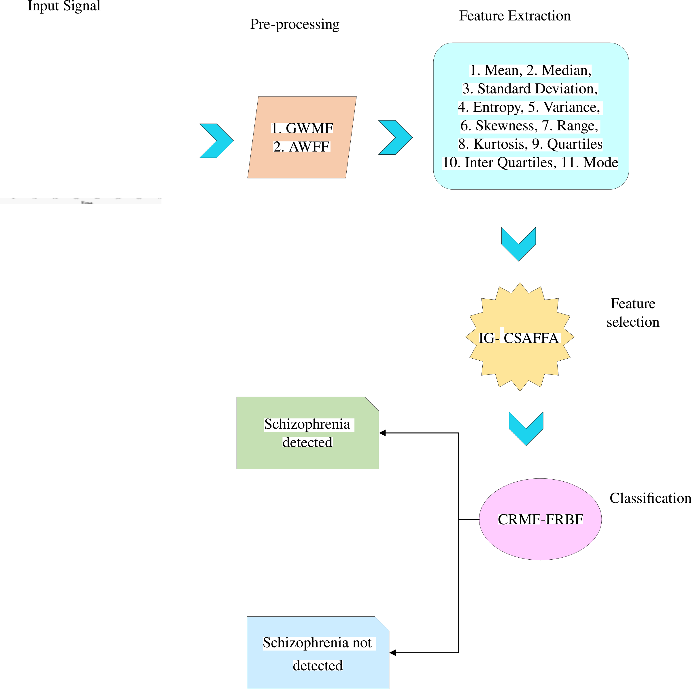
Schizophrenia is one of the severe mental illnesses where reality is seen in an aberrant manner. Schizophrenia results in profoundly abnormal thinking, delusions, and hallucinations, and it seriously impairs a person’s ability to carry out their daily tasks. Schizophrenia can lead to a variety of issues, including distorted thinking and behaviours. The study of brain activity is a significant topic of research in the field of human neuroscience. EEG data are frequently employed as a low-resolution diagnostic technique for general cognitive activity investigation. Understanding the abnormalities of brain illnesses, particularly schizophrenia, is made much easier by EEG readings. This study classifies EEG signals for schizophrenia. The block diagram of the proposed schizophrenia disease classification model is shown in figure 1.

Pre-processing

In pre-processing stage, the input signal is pre-processed using the GWMF and AWFF filters. The input signal having some noise content, so it is removed in this stage for obtain accurate results in the following stages.

Gaussian-Weighted Median Filter (GWMF)

An important challenge in medical imaging is removing noise from the source pictures. When using the noise reduction step, it’s best to retain the image’s clarity as much as possible while leaving the image’s edges alone. The average brightness values of the adjacent pixels are used to determine each output pixel in median filtering, a common low-pass filter that uses input pixels as the starting point. Additionally, the salt and pepper sounds may be effortlessly eliminated using a median filter. So, in this study, the preprocessing of the input photos was done using this filter.

Design a weighted filter where the central pixel has the highest weight (following a Gaussian distribution) and neighboring pixels have decreasing weights as they move away from the center. Then, use this weighted filter for filtering, where the median operation is applied with weights based on a Gaussian distribution. The median value of their neighbours is used to replace pixels in median filtering,

y_(m,n)=f(x)*median(x_ij:(i,j)∈τ) (1)

Where τ defines the nearby neighbors in (m, n) and f(x) is the Gaussian distribution function and which is described as,

f(x)=(1)/(√(2πσ²))e^{(-((x-μ)2)/(2σ2))} (2)

Where μ is the mean value, and σ is the variance.

Adaptive Weighted Fuzzy Filtering (AWFF)

The fundamental job of a fuzzy filter is to handle time-series signals by reducing noise, extracting significant features, or drawing inferences from fuzzy rules. Fuzzy rules are typically constructed using language variables and membership functions. Hybridizing fuzzy filtering with entropy-based filtering can be a powerful approach for image enhancement or noise reduction in digital images. Fuzzy filtering can help capture and represent uncertainty or ambiguity in pixel values, while entropy-based filtering can be used to make decisions based on the information content or randomness within a local region of an image.

According to the fuzzy theory, a membership or belonging function μ_A(x) describes the progressive belonging of element x to set A. If X is the set of all feasible items a fuzzy set A in X is defined as follows:

A=H(C)*{(x,μ_A(x)|x∈X} (3)

Where “membership function of the fuzzy set A” is μ_A(x) and H(C) is the entropy function. The filters used in fuzzy logic image processing model the collection of fuzzily defined attributes presents in the picture. The two types of uncertainty that have been recognized are vagueness and ambiguity. One of the most important aspects of the fuzzy theory are the inference rules that are directly applied to the pixels. The outputs of fuzzy inferential filters can be recognized using these principles. These sentences consist of a set of logical links and fuzzy conditional assertions, often known as IF-THEN statements. Some sample input signal with their pre-processed signal after applying the GWMF and AWFF are shown in figure 3.

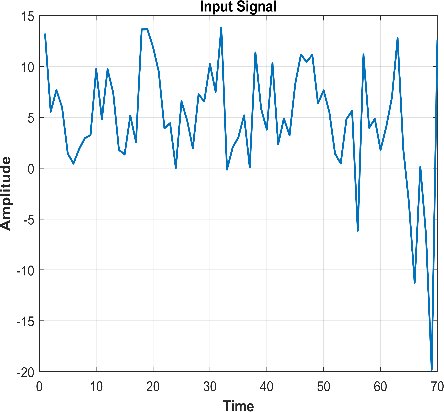
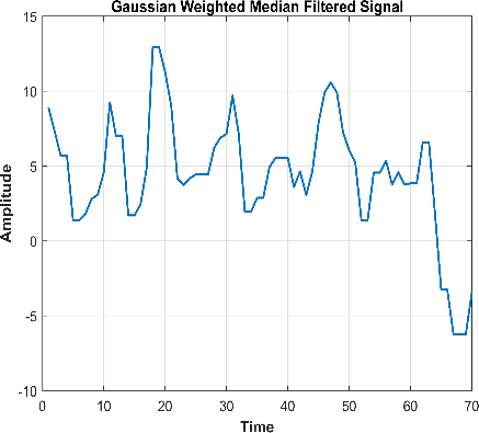
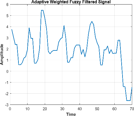
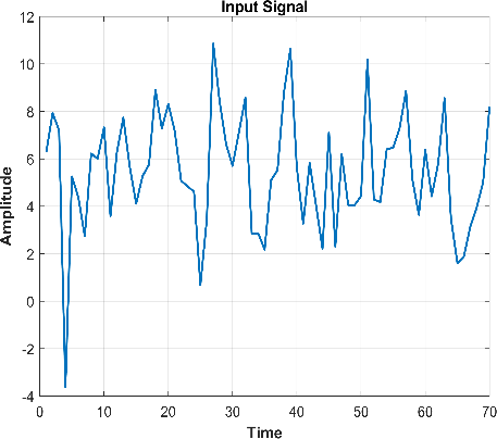
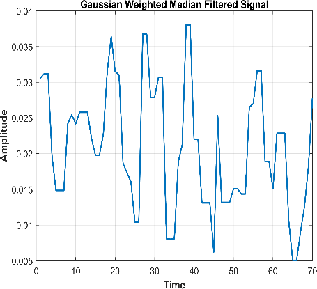
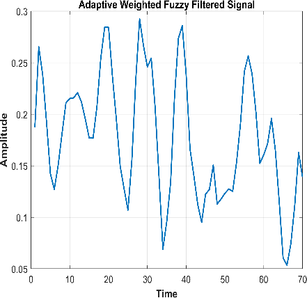
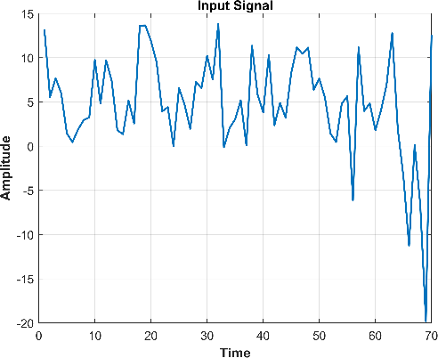
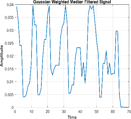
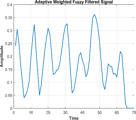
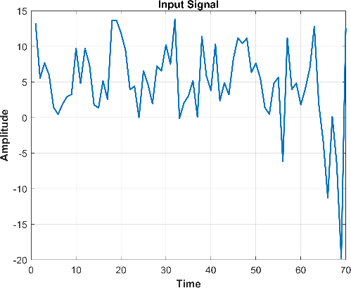
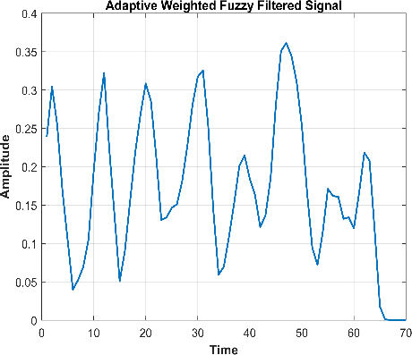
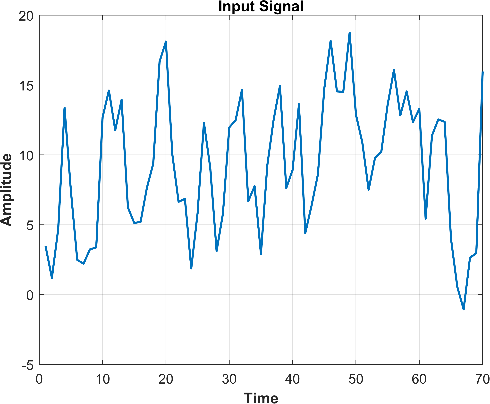
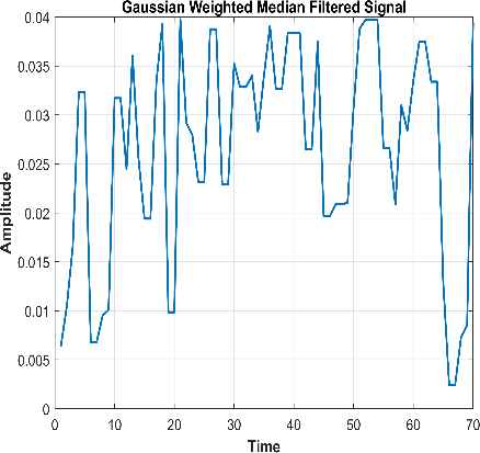
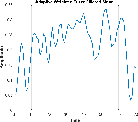
Figure 3: Preprocessed signal after applying GWMF and AWFF

Feature Extraction

To extract the features from the pre-processed signal, statistical methods such as the mean, median, standard deviation, entropy variance, skewness, range, kurtosis, Quartiles, Inter quartiles and mode are used.

Mean

The mean, often known as the average, is a statistic that illustrates the arithmetic mean of a set of data and acts as a measure of central tendency. It is calculated by taking the average of each variable in the dataset and dividing that number by the total number of variables.

Mean=(Sum of all values)/(Total number of values) (4)

Median

A different technique to express central tendency is to use the median, which represents the midpoint of an ordered set of data. The data is divided into two equal halves when half the numbers are below the median and the other half are above it. The median is less prone to outliers, or exceptionally high or low figures, in comparison to the mean. The definition of the median is,

Median={(l+1)/(2), for odd ; (l)/(2), for even (5)

Where l is the last number of the series.

Standard Deviation (SD)

A measurement of the data’s dispersion from the mean is referred to by the abbreviation SD (σ). When the standard deviation is low, the data are thought to be clustered around the mean, but when it is high, the data are widely spread.

SD (σ)=√((∑((x_i-μ)²))/(N)) (6)

Where x_i is the input variable, μ is the mean value and N is the total number of input variables.

Variance

The fluctuation between specific values in a data collection is statistically measured as variance. Consequently, the variance of a collection of integers is the difference among each number in the set and its mean (average), between each individual number in the set.

Variance=(∑((x_i-μ)²))/(N) (7)

Kurtosis

An indicator of how heavily or lightly tailed the data are in comparison to a normal distribution is the kurtosis statistic. In other words, data sets with an elevated kurtosis are more likely to have large outliers or massive tails. Light tails and few outliers are frequently found in data sets with low kurtosis. The worst-case scenario would be a distribution that is uniform.

Kurtosis=(4^thMoment)/(4^thMoment²) (8)

Skewness

By using a formula that multiplies the difference between the mean and median and divides the standard deviation by three, skewness is determined.

Skewness=(3(Mean-Median))/(SD) (9)

Entropy

Entropy may be used as a broad indicator of the quality of energy, with lower values indicating higher quality energy. In comparison to poorly organized energy storage, an efficient library has less entropy. The random-pile library is a method of energy storage with a high degree of unpredictability.

H(C)=-∑_i^c(P(c_i)log₂(P(c_i))) (10)

Where P_i is the number of values in the classification class equals the number of samples for classes i and c.

Range

The spread or diversity of values within a dataset may be quantified using a straightforward measurement known as range. The dataset’s highest and minimum values are divided to arrive at the difference. To get the range (R), use the following formula:

R=Maximum Value-Minimum Value (11)

Quartiles

The quartile formula may be used to split a piece of data into four equal halves. The first quartile lies between the first phrase and the median. The median is in the second quartile. The median and the last term meet in the middle, which is the third quartile. In mathematics, they are referred to as Eqs. (11), (12), and (13), respectively. When the observations are organized in ascending order, the quartiles are shown as follows:

First Quartile: Q₁= ((x+1)/(4))^thitem (12)

Second Quartile: Q₂= ((x+1)/(2))^thitem (13)

Third Quartile: Q₃= 3((x+1)/(4))^thitem (14)

The number of elements in a dataset is indicated by the letter “x”. The lower quartile is represented by the first quartile Q₁, while the median, or second quartile, Q₂, splits the data into two equal halves. The term “upper quartile” (Q₃) refers to the third quartile. The interquartile range, denoted as Q₃-Q₁, is used to calculate the difference between the upper and lower quartiles.

Inter quartile range (IQR)

The interquartile range, or IQR, which is the area between the first and third quartiles, is a commonly used statistic to represent variability in data sets including outliers. Q₁ stands for the first quartile, which is the portion of the data set that makes up 25% of the items below it. A result in a data set is said to be in the third quartile, or Q₃, if it accounts for 25% of the values above it. The interquartile range is defined by Eq. (15),

I_R= Q₃-Q₁ (15)

Mode

The mode in statistics is the value or values in a dataset that occur with the highest frequency, meaning it is the most frequently occurring value in the dataset. In other words, the mode represents the data point that appears most frequently. To find the mode, use the following Eq. (16):

M_o = {v₁, v₂, …, v_n} (16)

Where M_o represents the mode. v₁, v₂, …, v_n are the values in the dataset that occur with the highest frequency.

Feature Selection

A CSAFF with strong categorization performance is used to execute information gain. It is a commonly used entropy-based metric in the machine learning community. Information gain uses relationships between attributes and classifications as the basis for how it distributes feature weights statistically. Let S(s₁,s₂,…,s_n) be the group of n cases in a dataset, B(b₁,b₂,…,b_p) be the set of p attributes, and C(c₁,c₂,…,c_m) be the m categories and their collection. The number p(c_i) denotes the percentage of the i^th classes in S with the label c_i (i = 1, 2,…, m). The dataset’s entropy is provided by:

H(C)=-∑_i=1^m(p(c_i)log₂(p(c_i))) (17)

Every characteristic in the classification system for the data has an information gain (IG). The q^th attribute of the dataset, with q = 1, 2,…, p, is represented as B_q (b_q1, b_q2,…, b_qk). The appropriate conditional entropy for the property B_q is:

H(C|B_q)=-∑_j=1^k(p(b_qj))∑_i=1^m(p(c_i|b_qj)log₂(p(c_i|b_qj))) (18)

When b_qj is the value of the B_q attribute, which has k different possible values, and p(b_qj) denotes the prior probability of the categorical variable C. The equation p(c_i|b_qj). represents the conditional probability of the variable C following the application of the attribute B_q. The value of information gain for the attribute Aq is therefore provided by the difference between H(C), H(C|B_q), using the Eq. (19):

IG(B_q)=H(C)-H(C|B_q) (19)

Typically, more information acquisition indicates that a characteristic is essential for classification.

Objective Function

Finding the optimal feature subset with the fewest features and highest classification accuracy is what feature selection seeks to do for a given dataset. The performance of the classifier in classification is significantly influenced by both of these indicators in different ways. Here, using the same fitness function, we combine them into a single weighted indication that is shown in Eq. (20) below:

F_i=δ₁×A_Classifier+δ₂×(1-(S)/(P)) (20)

Where p denotes the overall number of attributes and s the number of attributes that were picked. In this case, δ₁ and δ₂ are equal to 1 and 0.001, respectively. Accuracy of the classifier’s classification is shown by the term A_Classifier, which can be found in Eq. (21).

A_Classifier=(K_c)/(K_c+K_i) (21)

Where, K_i and K_c stand for the number of occurrences that were successfully and wrongly classified. The fitness value can help to attain the objective of having a small number of features with the highest possible classification accuracy.

IG- CSAFFA

This section introduces the IG- CSAFFA feature selection approach. The first step is to initialize the population using the filter method IG. Then, to identify the ideal feature subset, we employ the CSAFFA method. The primary idea is to give each component a binary string to show if an attribute is picked; for example, a binary 1 means the feature is selected, whereas a binary 0 means it is not. The detailed description of the IG- CSAFFA algorithm is given below.

Mathematical modeling

In order to simulate the planned CSAFFA, this subsection provides mathematical models of a fennec fox’s natural behaviour.

Initialization

Fennec foxes serve as search members in the population-based metaheuristic algorithm known as CSAFFA. Each fennec fox in CSAFFA symbolizes a potential solution to the issue, and the decision variables’ values are determined by its placement in the search space. As a result, any fennec fox’s population is represented mathematically by a population matrix and expressed as a vector. In the search space, fennec foxes are first initialized at random using Eq. (22) at startup.

X_i😡_ij=lb_j+r.(ub_j-lb_j) (22)

Where i=1,2,…,N and j=1,2,….,m

Where X_i represents the i^th fennec fox, x_ij represents its j^th dimension (i.e., decision variable), N represents the total number of fennec foxes, m represents the number of choice variables, r represents a random number between [0, 1], and lb_j and ub_j represent the lower bound and upper bound of the j^th decision variable, respectively. A population matrix for the FFA made up of N fennec foxes is described in Eq. (23).

X=[[X₁] ; [⋮] ; [X_i] ; [⋮] ; [X_N]]_N×m=[[x_1,1 , … , x_1,j , … , x_1,m] ; [⋮ , ⋱ , ⋮ , ⋱ , ⋮] ; [x_i,1 , … , x_i,j , … , x_i,m] ; [⋮ , ⋱ , ⋮ , ⋱ , ⋮] ; [x_N,1 , … , x_N,j , … , x_N,M]]_N×m (23)

Where each column of the matrix X_i=(x_1j,x_2j,…,x_Nj)^T) represents a possible value for the j^th decision variable, and row X(x_i1,x_i2,…,x_im), the i^th row of the matrix X represents the i^th fennec fox in the population in the range N. After inserting the potential values suggested by each fennec fox into the Objective Function’s (OF) variables, the OF is assessed. In order to model the goal function’s estimated values mathematically, the vector mentioned in Eq. (24) is used.

F=[[F₁] ; [⋮] ; [F_i] ; ⋮ ; F_N]_N×1=[[F(X₁)] ; [⋮] ; [F(X_i)] ; ⋮ ; F(X_N)]_N×1 (24)

Where F_i is the value of the OF determined for the i^th fennec fox and F is the vector containing the OF’s values. Updates on the location of CSAFFA members in the search area were made using two typical fennec fox behaviours. Among them are digging in the sand to find things to eat and running away from predators.

Exploitation Phase 1: The sand-based digging to find prey

The search agent hunts alone in the midnight. It hunts its prey by digging with its feet after locating it using the strength of its huge ears to hear it beneath the sand. This search agent behaviour represents a local search, and by mimicking it, the CSAFFA may more effectively use its exploitation capacity to find a solution that is closer to the global optimum. A neighbourhood with a radius R surrounding the fennec fox’s real location is taken into consideration in order to replicate its behaviour while digging. A local search in this region by the fennec fox may lead to a more suitable answer. Eq. (25) through Eq. (27) are used to replicate this stage of upgrading CSAFFA members analytically.

x_ij^P1=x_ij+(2.r-1).R_ij (25)

R_ij=α.(1-(t)/(T)).x_ij (26)

X_i={X_i^P1, F_i^P1<F_i ; X_i, else (27)

Where R_ij is the neighbourhood radius for x_ij, t is the iteration count, T is the maximum iterations, and α is a constant set to 0. Where X_i^P1 is the new proposed status of the i^th fennec fox based on first phase, F_i^P1 is the value of its OF, x_ij^P1 is the its j^th dimension, and R_ij is the neighbourhood radius for X_i.

Exploration Phase: Cauchy-based Escape strategy

Wild predators including the striped hyenas, Pharaoh eagle-owl, and caracals are known to attack fennec foxes. This fennec fox’s escape maneuver serves as the foundation for the global search space scanning in our mathematical model. The suggested CSAFFA’s exploring power is increased by simulation of this escape plan. It facilitates finding the best global solution by not getting bogged down in the locally optimum areas. Because of this, the distribution of each candidate solution in the search space may be used as a model for the behaviour of the fennec fox as it tries to escape.

To improve the speed of the CSAFFA, the Cauchy-based Escape strategy is introduced. One common challenge in optimization algorithms is getting trapped in local optima. By introducing the Cauchy-based Escape strategy, fireflies have a better chance of escaping local optima because they have a higher probability of making larger jumps. This helps the algorithm avoid premature convergence and encourages the exploration of diverse solutions. Using Eq. (28) through (30), a mathematical simulation of the Cauchy-based Escape strategy of the CSAFFA population update is performed.

X_i^rand😡_i,j^rand=x_k,j∈k{1,2,…,N}and i=1,2,…,N (28)

x_i,j^P2={x_i,j+CM*r.(x_i,j^rand-I.x_i,j), F_i^rand<F_i ; x_i,j+CM*r. (x_i,j-x_i,j^rand), else (29)

X_i={X_i^P2, F_i^P2<F_i ; X_i, else (30)

Where CM is the Cauchy distribution function and it is given in Eq. (31) as,

CM=tan((π×(ε-(1)/(2)))) (31)

Where CM stands for a random value generated by the standard Cauchy distribution function’s inverse function and refers to a uniform distribution-generated random value in the range of 0 to 1. Then x_i,j^rand is the location where the escape is aimed towards the i^th search agent, F_i^P2 is the value of its OF, F_i^rand is the i^th OF value, X_i^P2 is the updated recommended status of the i^th search agent based on second phase, x_j^rand is the its j^th dimension, x_i,j^P2 is its j^th dimension, and i is a number chosen at random from the range 1 and 2.

After changing every fennec fox’s location in accordance with the first and second stages, the first CSAFFA iteration is finished. This updating procedure continues until the algorithm based on Eq. (28) to Eq. (30) has completed all iterations. After complete implementation, the CSAFFA offers a potential solution to the situation at hand. Algorithm 1 contains its pseudo-code of CSAFFA implementation phases.

Classification

A Convolutional Recurrent Median Filter with the Fuzzy Radial Basis function network (FRBF) is named as CRMF_FRBF is utilized for classifying the schizophrenia. CRMF_FRBF learning provides better classification by executing the hyper parameters tuning using a CSAFFA algorithm. The normal basic CNN model is used for performing this hybrid model. The deep learning models like CMRF and the FRBF are connected in serial connection. The pooling layer of the CNN is replaced with the Recurrent Median Filter (FMF) model for improving the pooling operation. After this layer the FRBF model is connected. Figure 3 depicts the proposed CRMF_FRBF model’s multilayered design.

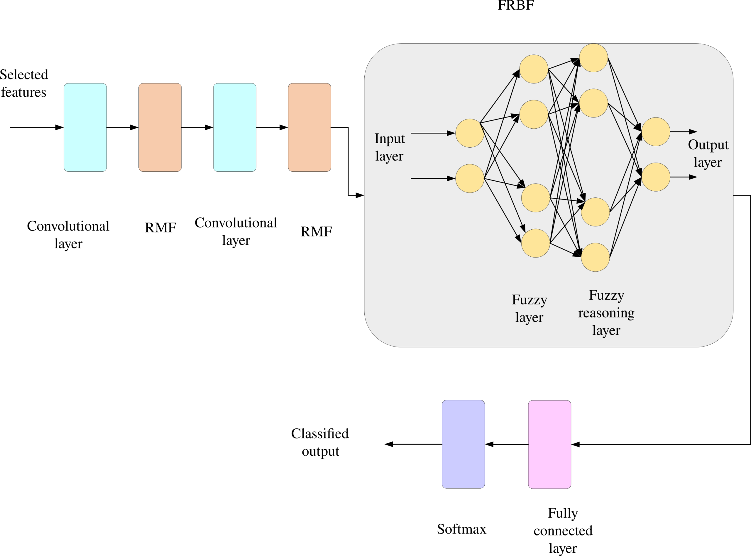
Figure 3: Structure of the CRMF_FRBF model

CRMF

CNN’s essential building pieces are convolutional, pooling, and one or more fully connected layers. It has three layered construction. CNNs have a data flow from input to output.

Convolutional layers: This particular layer serves as an extractor, therefore it aids in understanding how input pictures are represented. In feature maps, the neurons are organized. The set of trainable weights connects each neuron to the area of the previous layer, giving it the term “filter bank.” Using Eq. (8), the d^th output feature map for Co_d is calculated. INP is the input image, find stands for the convolutional filter linked to the d^th feature map, and stands for the 2D convolutional operator, which analyses every part of the input picture to determine the inner filter result. In addition, f(.) stands for the non-linear creation function. This makes it possible to extract the non-linear characteristics:

Co_d=f(fm_d*INP) (32)

Additionally, functions like the sigmoid and hyperbolic tangent are frequently used.

RMF

As a result, we integrated an RNN with the Median filter to significantly increase the method’s capacity for prediction in a nonlinear system. The method of filtering parameters was used as the LSTM network’s inputs, and the system was then able to output the expected value that was nearest to the actual value. The output of the Median filtering approach is given to the RNN model, based on RNN network rectification the pooling operation is performed. There are some important features are extracted form this stage.

Traditionally used RNNs combine supervised and unsupervised learning. This model’s input sequence data might have a length as long as its depth. The design of the RNN model consists of a feedback loop that connects each layer with the capacity to retain information from the previous input. As a result, it may make the model more trustworthy. In this model, x(t) is the input layer with index i at time t, and h(t- 1) is the hidden layer with index s at time t – 1. At time t, layer h(t) with index j is concealed. Y(t) is the output layer with index e at time t. The hidden layer with indexes i and j is connected to the input via the weight matrix U. Layers with the indices s and j are joined by the weight matrix W, that were previously concealed. The number of input units is m, and the weight matrix V connects the hidden layer and the output layer with the index j,e. There are n hidden units. There are k output units. The calculations of an RNN are governed by the following formulae. The input at the present step and the previously concealed state are used to determine h(t) in the first step:

h(t)=f(Ux(t)+Wh(t-1)) (33)

Where the nonlinear function f is one like tanh or ReLU. The first hidden state, which is commonly initialized to all zeroes, must be calculated using h(t-1). The output at step t is determined as y(t) in the second step using the formula:

y(t)=f(Vh(t)) (34)

For recurrent networks, the following formulas are used to derive h_j(t) and y_e(t):

h_j(t)=f(∑_i^m(x_i(t))u_ij+∑_sⁿ(h_s)(t-1)w_sj) (35)

y_e(t)=f(∑_j=1^k(h_j(t)v_je)) (36)

FRBF

A FRBF is made up of four layers: an input layer, a layer for fuzzying up the data, and a layer for fuzzy reasoning. Following the input components have been added to the input layer, they are moved to the layer of fuzzification, where they are connected to the layer of fuzzy logic, where the fuzzy rule checking is finished before the fuzzy calculation. The output and weighting of the output layer’s nodes follows. The architecture of the FRBF model is shown in figure 4.

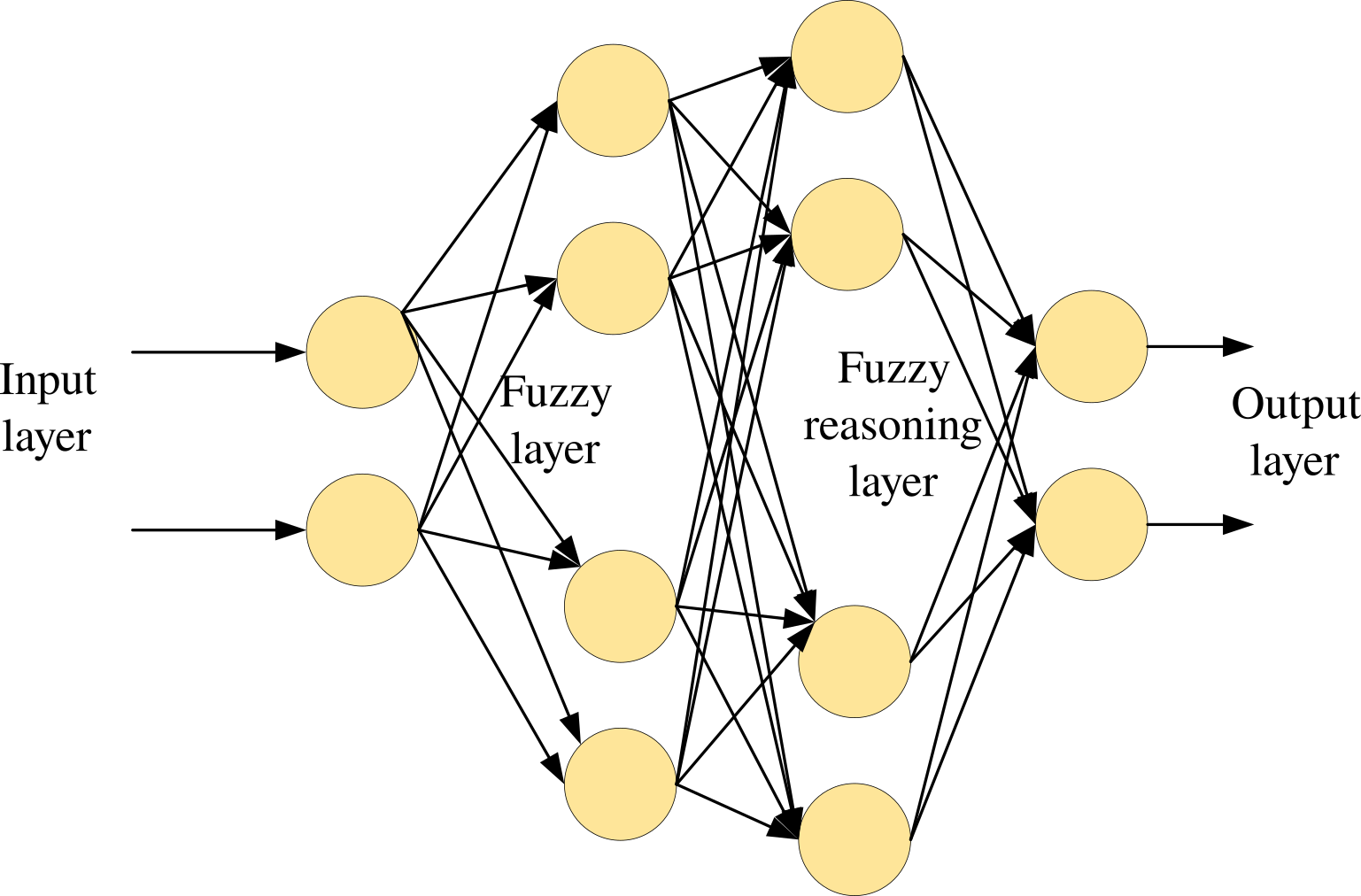
Figure 4: Layered architecture of the FRBF model

The input layer is the initial layer. Each node i in this layer may be represented by having the following input and output:

h₁(i)=x_i (37)

The layer of fuzzification is the second layer. This layer’s nodes each have a membership function that is a Gaussian basis function (b_j). Regarding the j^th node:

{h₂(i,j)=e^(net_j2) ; net_j²=(|x-c_ij|²)/(b_j²) (38)

Where b_j> 0 having the width of hidden layer neuron j and c_ij is the value of the central vector of the j^th neuron. fuzziness in reasoning is the third layer. Fuzzy rule matching and between-node fuzzy operations are made possible thanks to the layer’s connection to the layer of fuzzification. The product of this node’s input signals is what determines each node’s output, j:

h₃(j)=∏_j=1^N(h₂(i,j)) (39)

Where N=∏_i=1ⁿ(N_i )is the total number of nodes in the fuzzification layer and the i^th membership functions in the input layer. The final layer is called the output layer. The weighted sum of the input signals is what determines each node of this layer’s output:

h₃(l)=w.h₃=∑_j=1^N(w(l,j).)h₃(j) (40)

Where w is the relationship matrix among the output layer’s nodes and the third-layer nodes, and l is the number of output layer nodes. The FRBF is divided into four layers: an input layer, a layer of fuzzy reasoning, and a layer of fuzzy reasoning. The input can be defined as x=[s, ṡ] and the network’s output value, real value are thus represented by d̂(t)=h₄(l) and inaccuracy in the network’s estimate is:

ε₁(t)=d(ω_r,β,t)-d̂(t) (41)

The gradient descent approach is used to calibrate the changeable parameters. The definition of the desired function is:

E=(1)/(2)*ε(t)² (42)

Adjust the weights of the output layer is the FRBF’s learning method:

∆w(t)=-ϕ(∂E)/(∂w)=–ϕ(∂E)/(∂w)*(∂ε)/(∂d̂)(∂d̂)/(∂w) (43)

The output layer’s learning algorithm is composed of:

w(t)=w(t-1)+∆w(t)+α[w(t-1)-w(t-2)] (44)

Where α is the momentum factor, α ∈ [0, 1], and φ is the learning rate, [0, 1]. The following adjustments are made to the input layer’s membership function parameters:

{∆c_ij=-ϕ(∂E)/(∂c_ij)=-ϕ(∂E)/(∂net_j²)*(∂net_j²)/(∂c_ij)=-ϕδ_j²(1(x_i-c_ij))/(b_j²) ; ∆b_j=-ϕ(∂E)/(∂b_j)=-ϕ(∂E)/(∂net_j²)*(∂net_j²)/(∂b_j)=-ϕδ_j²(1(x_i-b_j))/(b_j²) (45)

Where δ_j²=(∂E)/(∂net_j²)=-ε(t)(∂d̂(t))/(∂net_j²) (46)

The procedure for mastering the parameters of a membership function is:

{c_ij(t)=c_ij(t-1)+∆c_ij(t)+α[c_ij(t-1)-c_ij(t-2)] ; b_j(t)=b_j(t-1)+∆b_j(t)+α[b_j(t-1)-b_j(t-2)] (47)

The FRBF system’s output from the aforementioned equation is:

d̂(t)=∑_j=1^N(w(l,j).h₃(j)=W^*Th(x)) (48)

Where W^* is the ideal network weight.

Fully Connected Layer

All of the inputs of the FC layer that forecasts the picture label are connected to all of the outputs of the layer before it. To anticipate the target class, this layer makes use of activation techniques such as softmax, sigmoid, etc. The output layer of a multi-classification model employs the Softmax function, which returns the probabilities of each class with a larger likelihood for the target class. The Softmax function offers a method for calculating discrete probability distributions over various classes, and the probabilities will all add up to one. Most binary classification models employ the sigmoid function, which outputs values in the range of 0 to 1.

SoftMax activation function

To anticipate the metaphor label sequences, we employ a thick layer with a softmax activation function. Because of the cost-sensitive cross entropy, our model’s loss function is constructed as follows:

L_softmax=-∑_sϵS(∑_i=1^N(ω_yiy_i)log((ŷ_i))) (49)

Where the projected value is y_i, the label for the i^th position is ŷ_i, and the loss weight is ω_yi.

Result and discussion

In this part, the results obtained using the proposed model are compared to those of the existing models. Performance metrics including sensitivity, specificity, accuracy, recall, precision, and F-Measure are produced in order to draw comparisons. The EEG based open source internet dataset is collected from Kaggle repository [26]. The implementation is performed using the Matlab tool.

Overall Comparison of the Proposed Classification Model

The proposed model is compared with the existing techniques like Convolutional Recurrent Neural Network (CRNN), RBN, Convolutional Neural Network (CNN), Long Short-term Memory (LSTM), and Gradient Recurrent Unit (GRU). The comparison table is shown in table 1.

Table 1: Performance evaluation of the suggested and current methods

The table provides a thorough evaluation of several machine learning or data analysis methods or models that have been used to a classification problem. A variety of crucial performance criteria are used to systematically compare these models. Notably, the “Proposed OIG_CRM_FRBN” model performs particularly well in a number of areas. It excels at successfully recognising affirmative situations, as seen by its sensitivity score of 98.81%, which highlights the dependability of its ability to detect the target condition. Additionally, the model shows outstanding specificity at 99.10%, demonstrating its competence in precisely recognising negative situations. With a 98.99% total accuracy rate, it is a solid option for this classification assignment due to the high degree of accuracy in its predictions. The model also claims an accuracy rating of 98.65%, which indicates that over 99% of its optimistic forecasts are accurate. The F-Measure of 98.73% demonstrates that it maintains an excellent balance between recall and accuracy. Additionally, it accurately detects genuine negative instances (99.21% NPV) and upholds low false positive (0.90%) and false negative (1.19%) rates, confirming its superior classification abilities. Finally, the MCC of 97.89% confirms the excellent calibre of classification performance displayed by this model. Other models, such as CRNN, RBN, CNN, LSTM, and GRU, perform significantly worse in comparison, making “Proposed OIG_CRM_FRBN” the best model for this particular classification job.

Sensitivity, sometimes referred to as True Positive Rate or Recall, assesses how effectively each method or model accurately detects positive cases. The “Proposed (OIG_CRM_FRBN)” approach in this table has the maximum sensitivity of 0.9881, which means that it accurately detects 98.81% of real positive instances. The other methods’ sensitivity values, which range from 0.9358 to 0.9693, are marginally lower. Specificity assesses how well each approach or model detects negative situations. The “Proposed (OIG_CRM_FRBN)” approach in this table has the greatest specificity of 0.9910, which means that it accurately recognises 99.10% of real negative situations. The specificity values for the other methods are likewise high, ranging from 0.9631 to 0.9809. Overall correctness is gauged by accuracy. The “Proposed (OIG_CRM_FRBN)” approach in this table has the greatest accuracy, 0.9899, which means that it properly categorises 98.99% of all instances. The accuracy values for the other methods are likewise high, ranging from 0.9547 to 0.9763. Figure 5 shows the comparison of the sensitivity, specificity and accuracy.

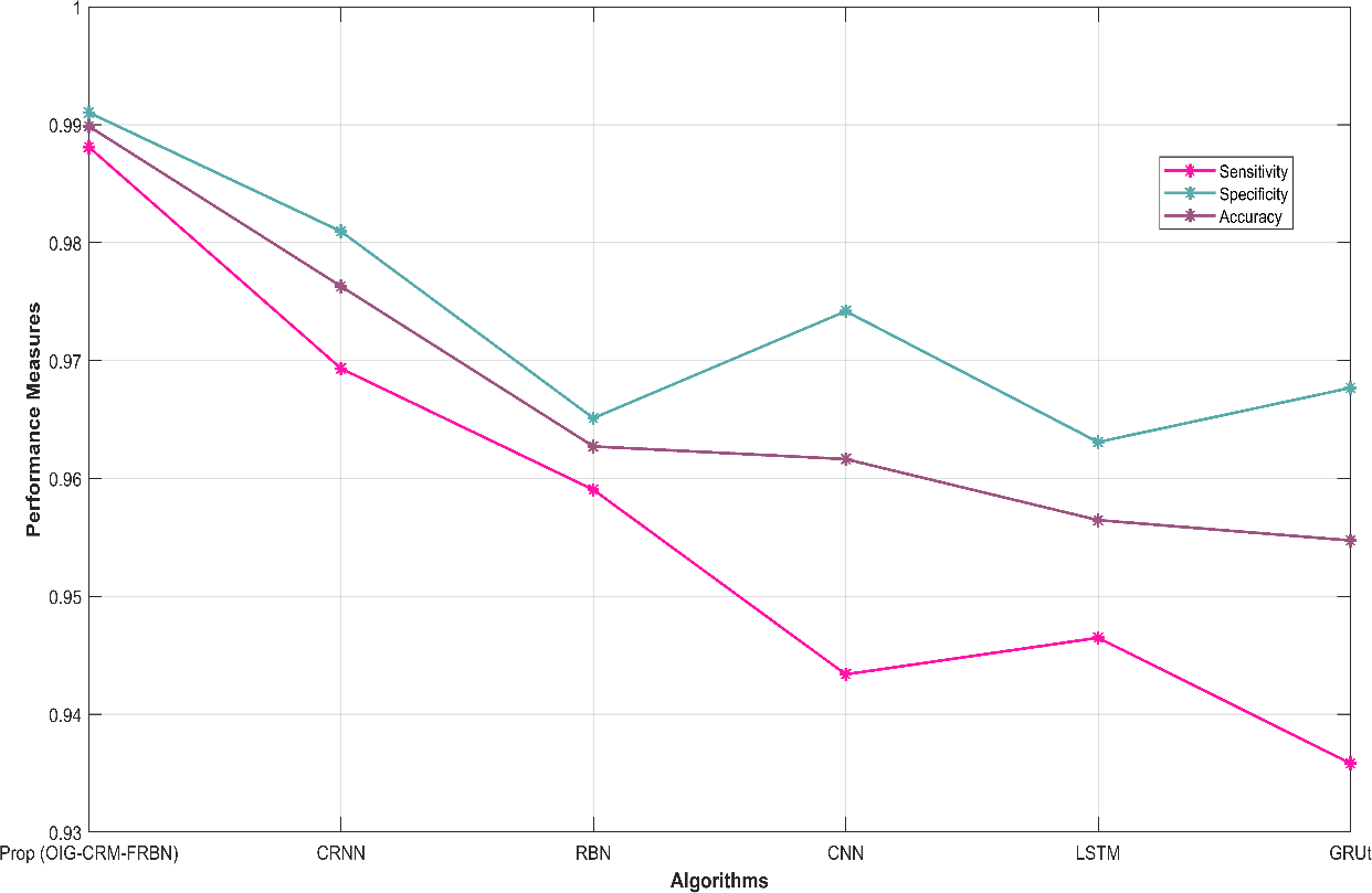
Figure 5: Comparison of sensitivity, specificity and accuracy

The degree of precision indicates how successfully a strategy or model avoids making incorrect predictions. The “Proposed (OIG_CRM_FRBN)” approach in this table has the highest precision, 0.9865, meaning that it predicts positive cases correctly 98.65% of the time. The accuracy ratings for the other methods, which range from 0.9444 to 0.9714, are likewise rather good. Recall, often referred to as sensitivity, is the same as what was previously said. It assesses how well each approach or model detects positive cases. The recall numbers in this table are consistent with the sensitivity levels discussed before. The harmonic mean of accuracy and recall is known as the F-Measure. The “Proposed (OIG_CRM_FRBN)” approach in this table has the greatest F-measure of 0.9873, demonstrating a balance between precision and recall. The F-measure values for the other methods are likewise good, ranging from 0.9439 to 0.9704. Figure 6 shows the comparison of the precision, recall and F-Measure.

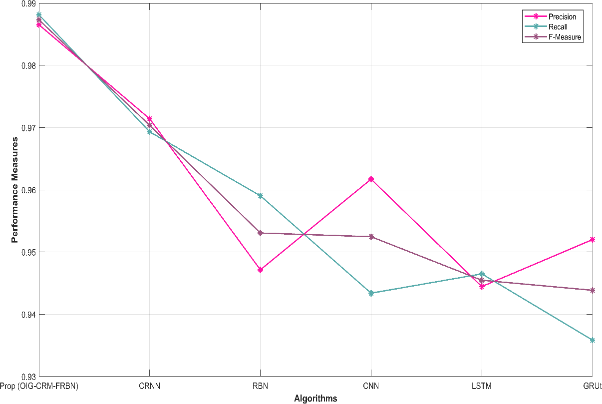
Figure 6: Comparison of precision, recall and F-Measure

NPV gauges each method’s ability to steer clear of unwarranted negative outcomes. The “Proposed (OIG_CRM_FRBN)” approach has the greatest NPV in this table, at 0.9921, meaning that it correctly predicts negative cases 99.21% of the time. With NPV values ranging from 0.9566 to 0.9795, the other methods are likewise quite effective. Information regarding real and fake positives and negatives is combined in the MCC measure. The “Proposed (OIG_CRM_FRBN)” method has the greatest MCC in this figure, at 0.9789, showing a high degree of agreement between predictions and results. With MCC values ranging from 0.9060 to 0.9506, the other methods are likewise effective. Figure 7 shows the comparison of the NPV and MCC.

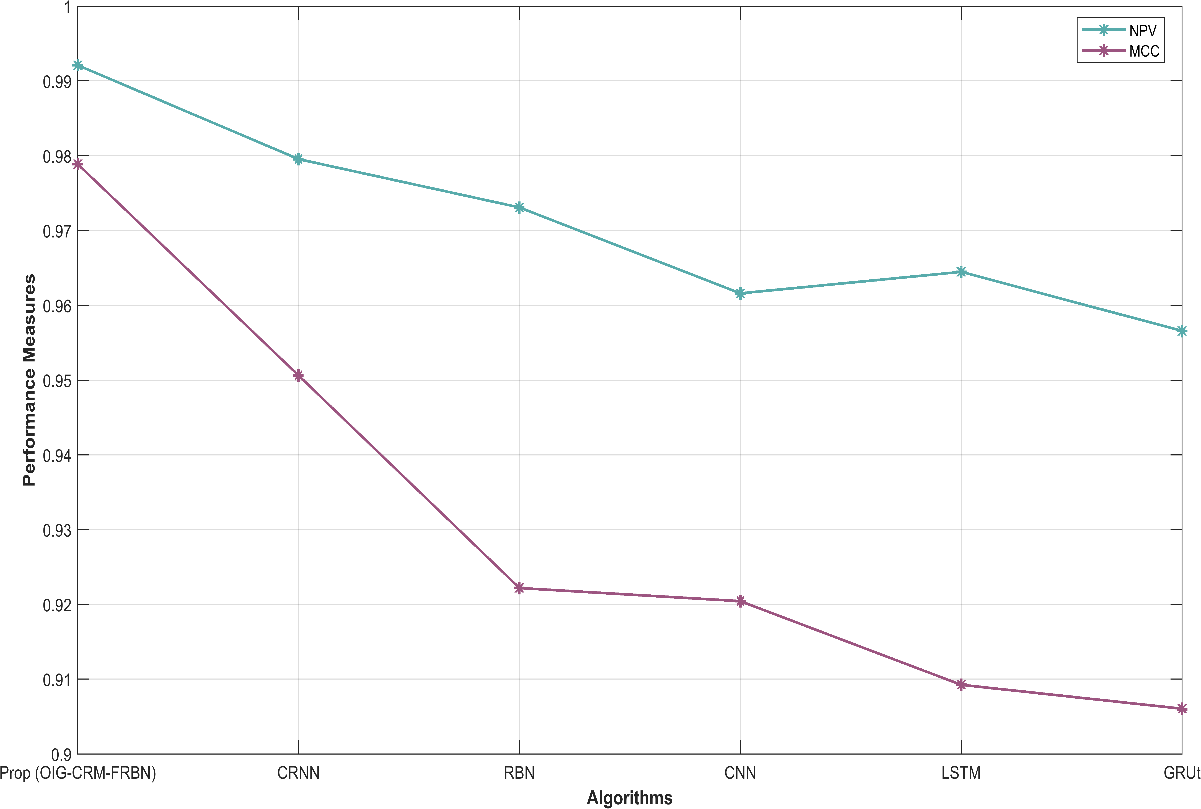
Figure 7: Comparison of NPV and MCC

The FPR quantifies the percentage of real negative cases that the model misclassified as positive. The “Proposed (OIG_CRM_FRBN)” method in this table has an extremely low FPR of 0.0090, suggesting that it seldom generates false positives. The FPR values for the other approaches are similarly rather low, ranging from 0.0258 to 0.0369. The fraction of true positive examples that the model misclassified as negative is measured by FNR. With an FNR of 0.0119, the “Proposed (OIG_CRM_FRBN)” method has an extremely low rate of false negatives. The FNR values for the other approaches are similarly quite low, ranging from 0.0307 to 0.0642. The FPR and FNR values are shown in figure 8.

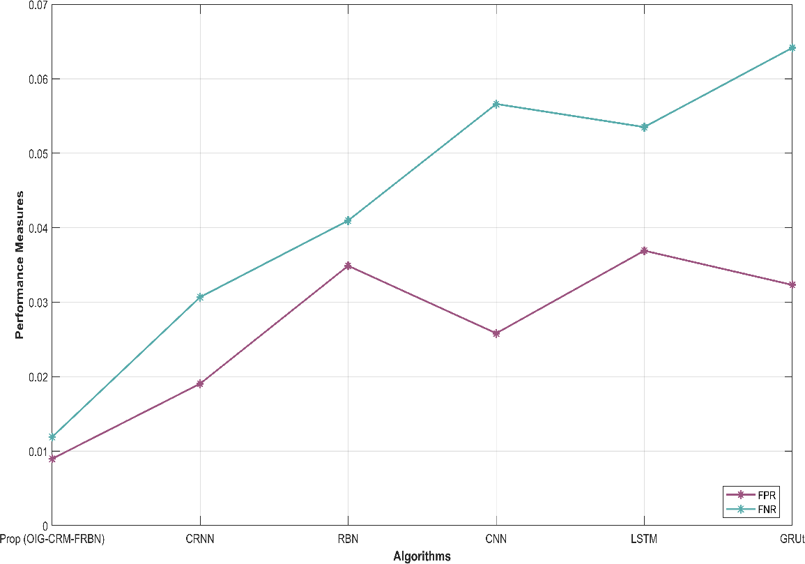
Figure 8: Comparison of FPR and FNR

The confusion matrix of the proposed model is shown in figure 9.

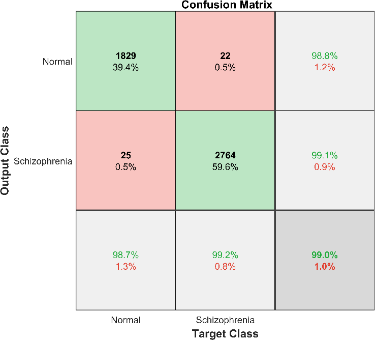
Figure 9: Confusion matrix for the proposed classification model

Conclusion

In conclusion, this research endeavors to address the intricate challenge of accurately diagnosing and classifying schizophrenia by harnessing the potential of EEG data. Our approach encompasses a meticulous two-tier preprocessing strategy, featuring GWMF and AWFF, which effectively enhance the quality of the EEG data for subsequent analysis. The extraction of a comprehensive set of statistical features ensures a rich representation of the preprocessed signal. Furthermore, we introduced a novel feature selection method named IG-CSAFF, to optimize the relevance of the selected features. The classification model CRMF_FRBF exhibits promising potential for improved schizophrenia classification. The use of CSAFF for hyperparameter tuning enhances the model’s performance. By amalgamating these advanced techniques, we aspire to significantly enhance the accuracy of schizophrenia classification, potentially advancing diagnostic capabilities and paving the way for more tailored treatment strategies in the field of mental health. In future work, integrating EEG data with other modalities such as functional MRI, genetic information, or patient demographics could provide a more comprehensive understanding of schizophrenia. Exploring fusion techniques and their impact on classification accuracy is a valuable avenue.

References

Caponnetto, P., Maglia, M., Mangione, M., Vergopia, C., Prezzavento, G.C., Polosa, R., Quattropani, M.C., DiPiazza, J. and Signorelli, M.S., 2022, November. Smoking Addiction in Patients with Schizophrenia Spectrum Disorders and Its Perception and Intervention in Healthcare Personnel Assigned to Psycho-Rehabilitation Programs: A Qualitative Research. In Healthcare (Vol. 10, No. 11, p. 2275). MDPI.

Pietrini, F., Tatini, L., Santarelli, G., Brugnolo, D., Squillace, M., Bozza, B., Ballerini, A., Ricca, V. and D’Anna, G., 2021. Self-and caregiver-perceived disability, subjective well-being, quality of life and psychopathology improvement in long-acting antipsychotic treatments: a 2-year follow-up study. International Journal of Psychiatry in Clinical Practice, 25(3), pp.307-315.

Agarwal, D., Kumar, A., BC, M., Kumar, V. and Sethi, S., 2021. Oral health perception and plight of patients of schizophrenia. International journal of dental hygiene, 19(1), pp.121-126.

Shoshina, I.I., Mukhitova, Y.V., Tregubenko, I.A., Pronin, S.V. and Isaeva, E.R., 2021. Contrast sensitivity of the visual system and cognitive functions in schizophrenia and depression. Human Physiology, 47, pp.516-527.

Berglund, A.M., James, S.H., Raugh, I.M. and Strauss, G.P., 2023. Beliefs About the Uncontrollability and Usefulness of Emotion in the Schizophrenia-Spectrum: Links to Emotion Regulation and Negative Symptoms. Cognitive Therapy and Research, 47(2), pp.282-294.

Walther, S., van Harten, P.N., Waddington, J.L., Cuesta, M.J., Peralta, V., Dupin, L., Foucher, J.R., Sambataro, F., Morrens, M., Kubera, K.M. and Pieters, L.E., 2020. Movement disorder and sensorimotor abnormalities in schizophrenia and other psychoses-European consensus on assessment and perspectives. European neuropsychopharmacology, 38, pp.25-39.

Bradshaw, N.J., Trossbach, S.V., Köber, S., Walter, S., Prikulis, I., Weggen, S. and Korth, C., 2020. Disrupted in Schizophrenia 1 regulates the processing of reelin in the perinatal cortex. Schizophrenia research, 215, pp.506-513.

Christensen, T.N., Wallstrøm, I.G., Eplov, L.F., Laursen, T.M. and Nordentoft, M., 2022. Incidence rates and employment trends in schizophrenia spectrum disorders, bipolar affective disorders and recurrent depression in the years 2000–2013: a Danish nationwide register-based study. Nordic Journal of Psychiatry, 76(3), pp.225-232.

Prabhakar, S.K., Rajaguru, H. and Kim, S.H., 2020. Schizophrenia EEG signal classification based on swarm intelligence computing. Computational Intelligence and Neuroscience, 2020.

Siuly, S., Khare, S.K., Bajaj, V., Wang, H. and Zhang, Y., 2020. A computerized method for automatic detection of schizophrenia using EEG signals. IEEE Transactions on Neural Systems and Rehabilitation Engineering, 28(11), pp.2390-2400.

Light, G.A., Joshi, Y.B., Molina, J.L., Bhakta, S.G., Nungaray, J.A., Cardoso, L., Kotz, J.E., Thomas, M.L. and Swerdlow, N.R., 2020. Neurophysiological biomarkers for schizophrenia therapeutics. Biomarkers in Neuropsychiatry, 2, p.100012.

Liu, F., Wang, L., Lou, Y., Li, R.C. and Purdon, P.L., 2020. Probabilistic structure learning for EEG/MEG source imaging with hierarchical graph priors. IEEE transactions on medical imaging, 40(1), pp.321-334.

Liang, J., Yu, Z.L., Gu, Z. and Li, Y., 2022. Electromagnetic Source Imaging via Bayesian Modeling With Smoothness in Spatial and Temporal Domains. IEEE Transactions on Neural Systems and Rehabilitation Engineering, 30, pp.2362-2372.

Poudel, G.R. and Jones, R.D., 2021. Multimodal Neuroimaging with Simultaneous fMRI and EEG. In Handbook of Neuroengineering (pp. 1-23). Singapore: Springer Singapore.

Chang, C. and Chen, J.E., 2021. Multimodal EEG-fMRI: advancing insight into large-scale human brain dynamics. Current opinion in biomedical engineering, 18, p.100279.

Prabhakar, S.K., Rajaguru, H. and Lee, S.W., 2020. A framework for schizophrenia EEG signal classification with nature inspired optimization algorithms. IEEE Access, 8, pp.39875-39897.

Ji, X., Quan, W., Yang, L., Chen, J., Wang, J. and Wu, T., 2020. Classification of schizophrenia by seed-based functional connectivity using prefronto-temporal functional near infrared spectroscopy. Journal of Neuroscience Methods, 344, p.108874.

Zou, H. and Yang, J., 2020. Multiple functional connectivity networks fusion for schizophrenia diagnosis. Medical & biological engineering & computing, 58, pp.1779-1790.

Ahmedt-Aristizabal, D., Fernando, T., Denman, S., Robinson, J.E., Sridharan, S., Johnston, P.J., Laurens, K.R. and Fookes, C., 2020. Identification of children at risk of schizophrenia via deep learning and EEG responses. IEEE Journal of biomedical and health informatics, 25(1), pp.69-76.

Hu, M., Qian, X., Liu, S., Koh, A.J., Sim, K., Jiang, X., Guan, C. and Zhou, J.H., 2022. Structural and diffusion MRI based schizophrenia classification using 2D pretrained and 3D naive Convolutional Neural Networks. Schizophrenia research, 243, pp.330-341.

Baygin, M., 2021. An accurate automated schizophrenia detection using TQWT and statistical moment based feature extraction. Biomedical Signal Processing and Control, 68, p.102777.

Baygin, M., Yaman, O., Tuncer, T., Dogan, S., Barua, P.D. and Acharya, U.R., 2021. Automated accurate schizophrenia detection system using Collatz pattern technique with EEG signals. Biomedical Signal Processing and Control, 70, p.102936.

Wang, K.Z., Bani-Fatemi, A., Adanty, C., Harripaul, R., Griffiths, J., Kolla, N., Gerretsen, P., Graff, A. and De Luca, V., 2020. Prediction of physical violence in schizophrenia with machine learning algorithms. Psychiatry research, 289, p.112960.

Chen, J., Li, X., Calhoun, V.D., Turner, J.A., van Erp, T.G., Wang, L., Andreassen, O.A., Agartz, I., Westlye, L.T., Jönsson, E. and Ford, J.M., 2021. Sparse deep neural networks on imaging genetics for schizophrenia case–control classification. Human brain mapping, 42(8), pp.2556-2568.

Chen, L., Li, Q., Song, H., Gao, R., Yang, J., Dong, W. and Dang, W., 2020. Classification of schizophrenia using general linear model and support vector machine via fNIRS. Physical and Engineering Sciences in Medicine, 43, pp.1151-1160.

Dataset is taken from https://www.kaggle.com/datasets/broach/button-tone-sz dated on 09/09/2023.

Editorial Staff

Academic Master Education Team is a group of academic editors and subject specialists responsible for producing structured, research-backed essays across multiple disciplines. Each article is developed following Academic Master’s Editorial Policy and supported by credible academic references. The team ensures clarity, citation accuracy, and adherence to ethical academic writing standards

Content reviewed under Academic Master Editorial Policy.

• Editorial Staff

  Grid-Connected Solar PV Systems and Power Quality Review
• Editorial Staff

  Predicting Cardiovascular Diseases with PCA and Artificial Neural Networks
• Editorial Staff

  Maternal and Neonatal Outcomes Following Water Birth Systematic Review and Meta-Analysis
• Editorial Staff

  Electrospun Polymeric Nanofibers for Biomedical Applications