
Abstract
Electroencephalography (EEG) is favoured for its cost-effectiveness and rapid response time in Brain-Computer Interface (BCI) applications. However, the selection of optimal EEG channels is crucial to maintain signal quality while minimizing preparation time and ensuring usability. Traditional manual channel selection based on neuroscientific knowledge may not always yield optimal results. This study presents an innovative approach for enhancing the efficiency and accuracy of BCI systems based on EEG data. The proposed methodology involves six key steps. Data Augmentation incorporates Synthetic Minority Over-sampling Technique (SMOTE) to enrich the dataset, improving its representativeness. Signal Pre-processing begins with notch filtering, Independent Component Analysis (ICA), time windows, Empirical Mode Decomposition (EMD) is introduced to capture underlying oscillatory components. Optimal channel selection introduces the new MothCray Optimization (MCO) model, a hybrid of Moth Flame Optimization (MFO) and Crayfish Optimization Algorithm (COA). Feature Extraction involves the extraction of various features from the selected EEG channels and Intrinsic Mode Functions (IMF), encompassing time-domain characteristics, frequency-domain attributes, connectivity measures, IMFs-based features capturing oscillatory patterns. Feature Selection introduces the hybrid optimization model MCO to enhance the feature selection process, striking a balance between exploration and exploitation. Classification via Spatio-Temporal EEGNet involves the development of a customized deep learning model known as Spatio-Temporal EEGNet. The proposed model is implemented using Python. In Dataset 1, the CNN achieved an accuracy of 0.98497, while in Dataset 2, it attained an accuracy of 0.986994.
Keywords – EEG; BCI; SMOTE; MCO; MFO; COA; EEGNet.
1. Introduction
Recent years have seen a fast increase in interest in the subject of brain-computer interface (BCI), which has the potential to completely alter how people interact with technology. Through the use of a BCI system, which establishes a direct line of communication between the brain and an external device, people are able to operate numerous technologies, such as prosthetic limbs, by simply thinking about them [1] [2]. The choice of suitable channels for recording brain signals is one of a BCI system’s most important elements. The electrical activity of the brain is measured using a non-invasive technique called electroencephalography (EEG) [3]. Multiple electrodes are positioned on the scalp to collect EEG signals, and the resulting data is utilised to decode the user’s intent. An integral part of creating a BCI system is choosing the channels for EEG data gathering [4] [5]. A channel is a particular scalp electrode that is used to record EEG signals. The system’s accuracy and dependability can be considerably impacted by the quantity and location of the channels utilised. Therefore, choosing the appropriate channels is essential to getting the greatest outcomes possible [6]. The position of the electrodes, the nature of the task, and the frequency band of interest are only a few of the variables that go into choosing the EEG channels for a BCI system. Usually, a subset of channels is chosen by researchers based on the brain areas that are most pertinent [7].
Channels over the motor cortex (located in the middle of the scalp) would be used if the BCI system’s objective was to identify motor imagery (MI). The type of work is equally as important to channel selection as the location of the electrodes. Different tasks involve the activation of various brain areas, necessitating the use of several electrode sets [8] [9]. For instance, electrodes would need to be placed over the occipital cortex, which is located at the rear of the scalp and is in charge of processing visual information, in order for a BCI system to detect visual inputs. The interest frequency band must be taken into account while choosing EEG channels [10] [11]. EEG signals can be broken down into various frequency bands, each of which corresponds to various states or activities of the brain. For instance, the beta band (12–30 Hz) is connected to muscular activity, while the alpha band (8–12 Hz) is connected to peaceful wakefulness. As a result, researchers can choose channels that are most responsive to the target frequency band [12]. Machine learning methods are now frequently utilised in BCI systems to analyse EEG data and interpret human intent.
To train the models for these strategies, a significant amount of high-quality EEG data is needed. In order to get precise and trustworthy findings, it is essential to use the right data gathering routes. A crucial step in creating a BCI system is choosing the EEG channels [13] [14]. When choosing channels, it is crucial to take into account the position of the electrodes, the nature of the task, and the interest frequency band. For the purpose of creating precise and dependable BCI systems, high-quality EEG data must be collected using the right channel selection [15]. The potential for BCI systems to enhance the lives of people with impairments or neurological illnesses is becoming clearer as a result of the ongoing developments in BCI technology and machine learning methods. The key contributions of this research are as follows:
To ensure robust signal pre-processing: Implementing a comprehensive signal pre-processing pipeline, including notch filtering to eliminate power line interference and ICA for artifact removal. Segmenting data into one-second time windows to align with motor imagery tasks and utilizing EMD to capture oscillatory components.
To optimize channel selection: Introducing the novel hybrid optimization model, MCO, which combines MFO and COA to optimize channel selection, ensuring only the most informative EEG channels are considered for analysis.
To enable comprehensive feature extraction: The feature extraction process encompasses various aspects, including time-domain features (mean, variance, skewness, kurtosis), frequency-domain features (power spectral density, spectral entropy, MEMD, connectivity measures (coherence, phase locking value), and IMF-based features, providing a representation of EEG data.
To improve feature selection: Introducing the innovative MCO method for feature selection, enhancing the efficiency of the classification model by selecting the most relevant features.
To propose classification via spatio-temporal EEGNet: The introduction of the novel spatio-temporal EEGNet, a dedicated classification model for AD diagnosis.
This article is categorized as: Section 2 deals with research gaps existing work of the presented model. Section 3 details the proposed methodology of the work, which is experimented with and analysed. Section 4 shows the result analysis and the comparative debate of this model. Section 5 gives the outcome of the work.
2. Literature Review
In 2019, Ko et al. [16] introduced a groundbreaking concept by harnessing the power of fuzzy integrals, specifically the Choquet and Sugeno integrals. These integrals offered a fresh perspective on data interactions within BCIs. The result was the creation of the multimodal fuzzy fusion-based BCI system. This system broke new ground by combining these integrals, resulting in remarkable performance enhancements. Moving to 2021, Deng et al. [17] recognized the growing influence of deep learning in BCI research, especially concerning MI-BCI. Although deep learning models had boosted accuracy, interpreting these models remained a challenge. The study introduced EEGNet, a deep learning model, and conducted a comparative analysis with the traditional Filter-Bank Common Spatial Pattern (FBCSP) algorithm. The study went further by unveiling the connections between EEGNet’s components and well-known techniques such as Discrete Wavelet Transform (DWT) and Common Spatial Pattern (CSP). To elevate EEGNet’s performance, they introduced Temporary Constrained Sparse Group Lasso (TCSGL). In the same year, Fumanal-Idocin et al. [18] delved into the realm of interval-valued moderate deviation functions. These functions offered a novel means of assessing similarity and dissimilarity among interval-valued data, which was particularly relevant in the context of motor-imagery brain-computer interfaces (MI-BCIs). The primary focus was on interval-valued moderate deviation functions that preserved the input interval widths. By employing fuzzy implication operators to quantify uncertainty in classifier outputs, these functions played a pivotal role in the decision-making phase of MI-BCI systems, enhancing their overall performance.
In 2019, Lazurenko et al. [19] brought forth an innovative neural network-based method to detect EEG patterns associated with motor imagery, representing mental equivalents of physical movements. This approach leveraged Local Approximation of Spectral Power with Radial Basis Functions (LASP-RBF) and introduced an original algorithm for interpreting neural network responses over time. The study introduced an asynchronous neural interface featuring a committee of three neural networks responsible for classifying EEG patterns related to upper and lower limb motor imagery. Shuailei et al. [20] focused on revolutionizing MI-BCI. Traditionally, BCIs decoded movements based on low-level command patterns, which limited users to a single imaginary command per body part. In this study, a novel high-level command pattern was introduced, combining hand movements in a way that opened up the potential for a broader range of tasks without compromising distinctiveness and stability. This groundbreaking concept laid the foundation for more intelligent and user-centric BCI systems. In 2021, Shi et al. [21] highlighted the pivotal role of channel selection in improving the performance of brain-computer interfaces (BCIs). Irrelevant and redundant channels were identified as key challenges, impacting classification accuracy, computational complexity, and BCI applications. The study introduced binary harmony search (BHS) as an innovative approach to optimize BCI channel selection. BHS was applied to training datasets to identify optimal channels, and their effectiveness was evaluated using test datasets. Leveraging common spatial pattern (CSP) features and employing sparse representation-based classification, linear discriminant analysis, and support vector machines, this approach significantly enhanced motor imagery (MI) classification.
Sun et al. [22] tackled the issue of accurate classification of MI-EEG tasks in BCI systems. EEG signal acquisition often involved a large number of channels, posing practical challenges. To address this, they introduced the EEG channel active inference neural network (EEG-ARNN), an end-to-end deep learning framework. This framework harnessed graph convolutional neural networks (GCN) to capture signal correlations in both temporal and spatial domains. It introduced two innovative channel selection methods, edge-selection (ES) and aggregation-selection (AS), which automatically identified optimal channels. This approach revolutionized BCI by enabling accurate classification with only a small subset of channels, reducing computational complexity, and streamlining applications. In 2020, Zuo et al. [23] introduced the Temporal Frequency Joint Sparse Optimization and Fuzzy Fusion (TFSOFF) method, a comprehensive solution for optimizing frequency bands and fusing classifications across multiple time windows. This approach involved segmenting EEG data into subtime windows, applying overlapping bandpass filters, and conducting feature extraction with common spatial patterns for each subband. Joint frequency band optimization was performed across multiple time windows using a joint sparse optimization model. The integration of fuzzy logic further improved MI analysis by effectively utilizing signals from various time periods.
In 2022, Moumgiakmas and Papakostas [24] conducted a thorough review of the field of Motor Imagery Brain-Computer Interfaces (MI-BCIs). This review, spanning from 2017 to the present, focused on the extraction of robust brainwave features capable of maintaining effectiveness across diverse subjects. While Common Spatial Patterns (CSP) methods received considerable attention, the review revealed the ascendancy of Wavelet Transform (WT). WT emerged as a robust choice, surpassing CSP and PSD methods in terms of accuracy and effectiveness across numerous datasets and recent works. The shift towards time-frequency features, notably in combination with Wavelet Transforms and deep learning, marked a significant trend in achieving impressive accuracy and robustness. In 2019, Togha et al. [25] addressed a fundamental challenge in EEG-based BCIs the limited spatial resolution of EEG due to volume conduction. They introduced the concept of Local Activities Estimation (LAE), a novel approach designed to enhance EEG’s spatial resolution. LAE achieved this by estimating the potential generated by sources proximate to an EEG electrode using a system of linear equations founded on specific definitions and assumptions. This innovative method elevated BCI system performance by overcoming spatial resolution limitations.
2.1. Problem Statement
The development of BCI systems faces a significant problem in the choice of optimal channels for EEG data recording [1]. The development of BCI technology can be hampered by improper channel selection, which can result in erroneous and unreliable findings. The position of the electrodes, the nature of the task, and the interest frequency band are only a few of the variables that go into choosing the EEG channels. Therefore, identifying the best channel selection strategies for obtaining high-quality EEG data becomes the problem statement for the development of the BCI system. This will make it possible to create precise and dependable BCI systems that can enhance the lives of people with impairments or neurological conditions. In order to collect the high-quality EEG data required for machine learning models to precisely decode user intent, it is crucial for the development of BCI systems to address the issue of appropriate channel selection [11].
3. Proposed Methodology
BCI-MI were developed via a novel deep learning-based approach. As the participant visualises limb motions, raw data from several scalp channels must be collected in order to identify motor imagery EEG signals. This approach improves the accuracy and efficiency of the BCI-MI process by adding deep learning techniques for channel selection and classification. The proposed model contains five main phases: (a) data gathering; (b) data augmentation; (c) signal pre-processing; (d) optimal channel selection; (e) feature extraction; (f) feature selection; and (g) classification. The overall designed architecture is shown in Fig. 1.
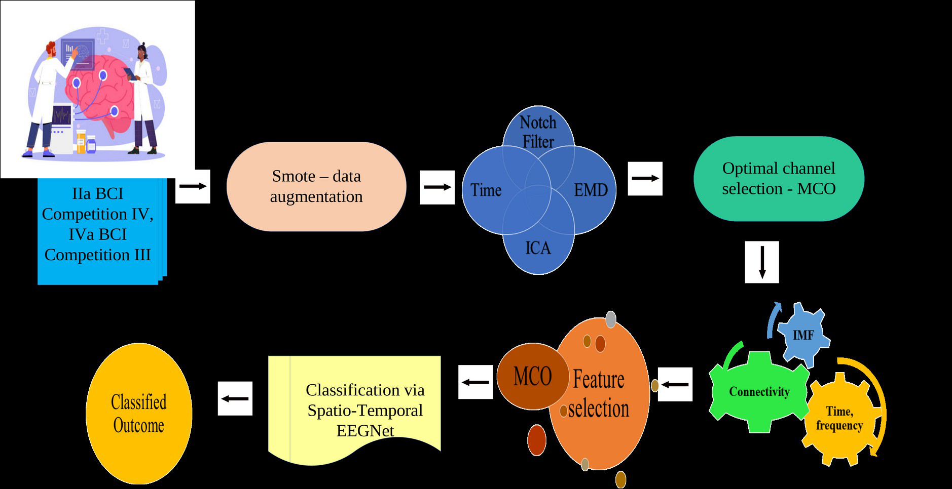
Figure 1: Overall proposed architecture
3.1. Data Collection
Two datasets—Dataset IIa BCI Competition IV and Dataset IVa BCI Competition III—are used in the study. While Dataset IVa has 59 channels, Dataset IIa only has 22. A SMOTE-based data augmentation strategy is used to lessen class imbalance. By creating artificial samples for the minority class, this technique balances the dataset. The core EEG dataset initially consists of 25 EEG channels. However, as these channels are Electrooculography (EOG) channels and are regarded as artefacts, they are not included in the rest of the investigation. As a result, the remaining 22 channels are put to use for further processing, and the dataset’s performance and balance are improved via SMOTE-based data augmentation.
3.2. Data Augmentation – SMOTE
The use of SMOTE-based data augmentation is a useful strategy for addressing the class imbalance in datasets. In order to minimise the randomness produced during the SMOTE process and subsequently reduce the variation associated with SMOTE-based oversampling, robust SMOTE-based oversampling approaches were developed. This method follows a number of standard steps, including calculating the necessary number of synthetic instances, choosing initial minority class instances for synthetic generation, selecting nearby minority class instances, and deciding on the interpolation method for generating new synthetic instances. By generating synthetic data points for the minority class based on Euclidean distances from their closest neighbours in the same class, SMOTE achieves oversampling. Since they are built using the original features, these freshly produced instances maintain similarities to the original data. It’s crucial to keep in mind, though, that SMOTE might not be the best option for high-dimensional data because it might inject more noise into the dataset. SMOTE is a strong tool for handling class-imbalanced data, although its usefulness can change depending on the details of the dataset, especially in high-dimensional situations.
3.3. Pre-Processing
The preprocessing stage receives the augmented signals as input. Several crucial actions are conducted during the signal pre-processing phase. To start, a notch filter is used to remove any power line interference that may have been present. The removal of artefacts like eye blinks and muscle activity is then accomplished using ICA. Following this, the EEG signals are divided into 1-second time windows, a practice for motor imagery tasks. In order to improve the data for future analysis, EMD is used to deconstruct the EEG signals and capture underlying oscillatory components.
3.3.1. Notch Filtering
Band-stop or band-reject filters, commonly referred to as notch filters, are specialised elements used in signal processing that target and exclude particular frequency ranges while allowing all other frequencies to pass through. They work by introducing a notch in the frequency response precisely at the unwanted frequencies. Imagine a scenario where a signal is interfered with at specified frequencies, like power line interference at 50 or 60 Hz. In order to solve this problem, notch filters block or weaken certain conflicting frequencies while maintaining the remainder of the signal. The LC notch filter, one of the most popular varieties of notch filters, uses inductors and capacitors to produce a frequency notch. Specific frequencies can be zeroed out by the LC filter, thereby removing them from the signal path, by carefully choosing the values of these components. Another variation uses digital signal processing methods, digital notch filters to generate comparable effects. To digitally cut notches in the frequency response, they employ algorithms like the infinite impulse response (IIR) or finite impulse response (FIR) filter.
3.3.2. Artifact Removal with ICA
The removal of unwanted artifacts that can contaminate the data, such as eye blinks, muscle activity, and other sources of non-brain-related noise. ICA is a commonly used technique for this purpose. ICA is a powerful statistical method used for disentangling a complex multivariate signal into its underlying, independent subcomponents. Its primary aim is to convert a set of observed signals, into a new set of maximally independent signals or components. ICA works by decomposing the recorded EEG signals into their underlying components, some of which may represent genuine brain activity, while others capture various artifacts. By analysing these components, ICA can effectively separate the EEG data into its constituent sources, making it possible to identify and remove those components associated with artifacts. Additionally, to facilitate further analysis and classification, the EEG signals are segmented into equal time windows, typically of 1-second duration. This segmentation allows researchers to work with smaller, more manageable portions of the EEG data, making it easier to apply various processing techniques and analyze brain activity during specific time intervals. The basic formula for ICA can be represented as per Eq. (1).
(1)
Where: denotes independent source components to extract, for the mixed data that was recorded from various sensors, and for the demixing matrix that changes into .
3.3.3. Segmentation into Time Windows
A key technique in time-series analysis is time-series segmentation, which aims to reveal a time-series’ inherent properties. Segmenting an EEG signal into equal 1-second time windows is a common approach used, particularly in motor imagery tasks. This method permits the analysis of localised brain activity patterns across time by discretizing the continuous EEG data. It promotes event-related potential analysis, supports feature extraction, makes noise reduction easier by separating troublesome regions, and improves brain dynamics interpretation. This segmentation technique is essential for learning about how the brain works, notably in BCI and cognitive study.
3.3.4. EMD on Segmented Data
To break down complicated signals into their individual oscillatory components, or IMF, EMD is a data-driven signal processing technique. EMD is extremely useful in many scientific domains since it is particularly good at studying signals with non-linear and non-stationary behaviour. The adaptability and adaptiveness of EMD is its basic tenet. EMD calculates IMFs directly from the input signal, as contrast to conventional approaches that rely on predetermined basis functions. Even when the signal’s properties change over time, its adaptability enables it to find hidden patterns and structures in the data. In the EMD procedure, IMFs are frequently found in the signal and extracted using a filtering process. Each IMF, which is arranged by frequency from high to low, represents an oscillatory mode that is present in the data. EMD offers a multiresolution perspective of the data by breaking down the signal into these IMFs, exposing underlying oscillations and trends that can be obscured by noise or complexity. It is especially useful in the analysis of EEG signals because it can record patterns of brain activity and help with the diagnosis of neurological illnesses.
3.4. Optimal Channel Selection
The goal of the channel selection method is to determine which channels will best convey the subject’s purpose during motor imagery tasks. The strategy overcomes the difficulty of simultaneously optimising various objectives, such as channel relevance and redundancy, by utilising multi-objective optimisation techniques. The suggested strategy improves the overall accuracy and resilience of the BCI system by repeatedly assessing each channel’s performance and choosing the most important ones. By excluding distracting or irrelevant channels, it may concentrate on those that offer the most accurate data on motor imagery. The next step is to continue processing and feature extraction using the chosen channels. The BCI system can better record and analyse the brain activity related to motor images through improved channel selection processes. As a result, categorization outcomes are more accurate and trustworthy, making it possible to precisely translate the subject’s intention into control orders for external devices. By maximising the selection of instructive EEG channels, the adjustment to the channel selection procedure improves the functionality of the motor imagery BCI system. By enhancing the system’s capacity to distinguish between various motor imagery tasks, it makes it possible to more precisely and consistently operate external devices using the subject’s brain activity. This research has established a novel strategy to enhance the channel selection process. For the purpose of selecting the best channels, the research uses a novel multi-objective hybrid deep learning approach called MCO. This strategy combines MFO and COA.
3.4.1. MothCray Optimization (MCO)
The MCO algorithm is a novel hybrid strategy that combines the MFO and COA and is inspired by the foraging and navigational strategies of crayfish and moths, respectively. The concept of transverse orientation from moths is retained by MCO, but it is modified for the optimisation context to avoid pre-convergence and guarantee a broad and exploratory search. With the use of foraging techniques inspired by crayfish, it effectively investigates the search space. Similar to how crayfish can survive in a variety of temperatures, MCO is flexible to changing problem environments, making it useful for solving challenging and dynamic optimisation scenarios. MCO excels in optimising a variety of problems, delivering improved solution quality and convergence time by constantly adjusting its exploration-exploitation balance and avoiding premature convergence.
Step 1: Initialization – Each crayfish in the multidimensional optimisation problem is a matrix with . A problem solution is represented by each column of the matrix. Each variable in the set of variables must be located between the top and lower bounds. As part of its initialization, COA creates a set of potential solutions called at random. Based on population size and dimension , candidate solution is proposed. Eq. (2) illustrates how the COA algorithm is initialised.
(2)
represents the initial population position, with indicating the population count, denoting the population dimension, and signifying individual position in dimension , determined via Eq. (3).
(3)
where is a random integer, is the lower bound of the dimension, and is the upper bound of the dimension.
Step 2: Fitness Computation – Fitness computation in MCO algorithm involves evaluating the fitness function for each individual in the population, quantifying the performance or quality of their solutions to the problem at hand. The fitness function can be a mathematical formula, simulation, or any other measure specific to the problem, guiding the optimization process towards finding better solutions. It is calculated as per Eq. (4).
(4)
Step 3: Define crayfish temperature and intake – Temperature plays a crucial role in crayfish behavior, influencing their activity and feeding patterns and given by Eq. (5). When temperatures exceed 30 °C, crayfish tend to seek cooler locations for summer shelter. In the ideal temperature range of 25 to 30 °C, crayfish actively engage in foraging. Their feeding quantity is temperature-dependent, following an approximate normal distribution. This means that temperature affects their feeding behavior, with the strongest foraging observed between 20 and 30 °C. COA defines the temperature range as 20 to 35 °C to account for this behavior. The mathematical model for crayfish intake is represented in Eq. (6), capturing the relationship between temperature and feeding patterns.
(5)
where, denotes the ambient temperature where the crayfish is situated.
(6)
Among them,and are employed to regulate the intake of crab at various temperatures. refers to the temperature that crabs like.
Step 4: Summer exploration stage for crayfish – Exploration (proposed) – The temperature is too high when The crayfish decides whether to spend the summer in the cave. Eq. (7) defines the cave.
(7)
where denotes the ideal position of the current population and denotes the best position so far determined by the number of iterations. The competition among crayfish for caves follows a random process. When a random number, represented as , is less than 0.5, it indicates that there are no other crayfish competing for caves. In such cases, the crayfish immediately enters the cave for their summer vacation. This behavior is influenced and enhanced by a logarithmic spiral, which is incorporated into MFO algorithm, guiding the crayfish towards the cave entrance in a spiral pattern during this phase of their activity, as per the proposed Eq. (8).
(8)
is a reducing curve, as stated in Eq. (11), where is the current iteration number and is the next generation iteration number. is the spiral function, and is a constant for defining the logarithmic spiral’s shape.
Step 5: Competition (Exploitation) – When and , defines other crayfish are also interested in the cave. At this time, they will fight to get the cave. The crayfish competes for the cave through Eq. (9), where represents a random crayfish individual, as shown in Eq. (10). During the Competition stage, crayfish compete and adjust their positions based on another crayfish’s position, expanding the search range of COA and enhancing the algorithm’s exploration ability.
(9)
(10)
Step 6: Foraging (Exploitation) – When the which is suitable for crayfish feeding, they will move towards the food source. Upon finding food, crayfish assess its size. If it’s too large, crayfish use their claws to tear it into smaller pieces and then consume it with their second and third walking feet. The food’s location is denoted as and shown in Eq. (11).
(11)
Food size is expressed as per Eq. (12),
(12)
Where denotes the ftness value of the crayfish and is the ftness value of the food location, and denotes the food factor, indicating the greatest food, and its value is constant 3. The largest food is used by the crayfish to judge the size of other foods. indicates that the portion size is excessive. The crayfish will now use its first claw foot to tear the food and given as per Eq. (13).
(13)
The second and third paws will alternately pick up the food and place it into the mouth once it has shrunk and become smaller. The combination of the sine function and the cosine function is used to replicate the alternating process. As per Eq. (14), foraging is as follows because, in addition, the food that crayfish obtains is related to the food that they consume.
(14)
When , the crayfsh just needs to move towards the food and eat directly, Eq. (15) is as follows,
(15)
Depending on the amount of their meal , crabs adopt a variety of feeding techniques throughout the foraging stage, with food serving as the best option. The crayfish will approach the meal when it is the right size for them to eat. A significant difference between the chaotic and ideal solution is present when is too large. As a result, needs to be smaller and closer to the food. regulate the food intake augmentation algorithm for crayfish’s unpredictability. Through the foraging stage, COA will move closer to the ideal solution, improving the algorithm’s capacity for exploitation and enabling strong convergence.
Step 7: Termination – Until a specific termination condition is fulfilled, the MCO algorithm iterates through the search, update, and evolution stages. This requirement could be the completion of a predetermined number of iterations, attaining a specific degree of fitness, or the convergence of solutions. The process is ended after the termination condition is met, and the algorithm completes its execution.
3.5. Feature Extraction
3.5.1. Time-domain features
Mean – It is defined as the total number of elements divided by the total number of elements in a set. Calculating the mean gives us a good understanding of the entire set of data. Consequently, the mean formula is calculated as per Eq. (16) and Eq. (17).
(16)
(17)
Where, = mean value, = Items given, = Total number of items
Variance – Analytically, the variance of a data set is the measure of numerical variation. Variance, in particular, determines how far off each integer in the set is from the mean and, consequently, from the other numbers in the set. This is mathematically shown in Eq. (18).
(18)
Skewness – A statistical measure known as skewness identifies an asymmetrical distribution of values. It gauges how far the numbers deviate from the mean by tilting them to one side or the other. The values in a normal distribution are symmetrical around the mean because the skewness is zero. Having a positive skewness implies that the values are moved to the right or that the right side of the distribution has a long tail, whereas having a negative skewness suggests that the values are shifted to the left or that the left side of the distribution has a long tail. According to Eq. (19), skewness is a term used to describe the distribution of data and to pinpoint any asymmetries in the data.
(19)
Kurtosis – Kurtosis is a statistical measure that describes the shape of the distribution of a set of values. It is a measure of the “peakedness” or “flatness” of the data compared to a normal distribution. A normal distribution has a kurtosis of zero, while positive kurtosis indicates a more peaked distribution and negative kurtosis indicates a flatter distribution. Kurtosis is commonly used in financial and economic analysis to describe the distribution of returns from investments or financial assets. In these applications, kurtosis is used to assess the risk associated with the investment, as high kurtosis may indicate a higher level of tail risk, or the risk of extreme outcomes, such as large losses. This is mathematically shown in Eq. (20).
(20)
3.5.2. Frequency-domain features
3.5.2.1. PSD
PSD is a popular feature extraction technique in signal processing, particularly in the analysis of EEG signals. PSD describes the power distribution of a signal across different frequency bands. It is calculated by taking the squared magnitude of the Fourier transform of the signal. PSD is used to extract important features of the EEG signal related to different brain activities, such as alpha, beta, gamma, and delta waves.
Welch Method
The frequently used Welch technique separates the signal into overlapping segments and averages the periodogram estimates of each segment in order to obtain a smoother PSD estimate. It is a common technique for figuring out a signal’s PSD from its broken-down components. This method involves averaging the periodogram calculations of each segment to deliver a smoother and more accurate PSD estimate. The Welch approach is described mathematically in the following.
Let be the discrete time-domain signal of length .
Divide the signal into overlapping segments of length and apply a window function to each segment.
Compute the periodogram estimate for each segment as per Eq. (21).
(21)
where is the sample of segment , FFT denotes the Fast Fourier Transform, is the Fourier transform of the window function , and denotes the magnitude squared. Average the periodogram estimates of all segments to obtain the final PSD estimate as per Eq. (22).
(22)
where denotes the sum over all segments.
3.5.2.2. Spectral Entropy
Spectral entropy measures the complexity or irregularity of a signal’s power spectrum. It quantifies how diverse the signal’s frequency components are. High spectral entropy indicates a diverse and complex spectrum, while low spectral entropy suggests a more ordered and regular distribution of frequencies. It is a measure of the spectral complexity of an EEG signal. It is calculated by multiplying the power in each frequency component by the logarithm of the same power and then summing these products. It quantifies the diversity of frequency components in the EEG signal, providing insights into its spectral characteristics expressed as per Eq. (23).
(23)
Shannon’s Entropy is a measure used to assess data spread and the dynamical order of a system. It quantifies the level of uncertainty or disorder in a dataset and is well-suited for normal distributions. However, it has limitations, including the potential loss of information through aggregation, the risk of overestimating entropy with excessive zones, and the inability to capture temporal relationships in time series data. These drawbacks need to be considered when applying Shannon entropy in data analysis.
3.5.2.3. Memd
Empirical mode decomposition (EMD), a data-adaptive multiresolution method, can be used to partition a signal into physically meaningful parts. EMD can be used to examine non-stationary and non-linear signals by breaking them down into their component parts at different resolutions. In multivariate EMD decomposition, IMFs from each IMF group that have the same order combine to generate a matrix. Correlations between matrices were employed to generate the fault correlation factor (FCF), utilising an integral technique, in order to find the effective IMFs integrating fault information. The standard EMD can only be utilised with signals that have a single variable. However, it is not possible to specify the local maxima and minima for multivariate signals explicitly, and it is also difficult to comprehend how oscillatory mode defines a multivariate IMF. This problem is addressed by interpolating the extrema of signal projections in different p-dimensional space directions. The result is a large number of p-dimensional envelopes. The average of these envelopes is then used to produce the local multivariate mean.
Let denotes the -variate signal, and denotes the projection vector along the direction indicated by angle on a sphere. MEMD divides a -variate signal into two parts using a vector-valued version of classic EMD as per Eq. (24).
(24)
where denotes the sets of IMFs are produced by the application of EMD, is the residue of monotonic, the scale-aligned intrinsic joint rotational modes in the -variate multivariate intrinsic mode functions (MIMF), , are present.
3.5.3. Connectivity measures
Phase-synchronization estimation techniques utilised in EEG and neuroimaging studies include coherence and phase locking value (PLV). Although they measure the synchronisation or connection between various brain regions similarly, they deliver data with varying degrees of granularity.
Coherence: Coherence provides a measure of the synchronization strength between two EEG signals at specific frequency points. It quantifies both the phase and magnitude consistency between these signals within a predefined frequency range. Coherence results in a single value for each frequency, indicating the overall degree of synchronization at that particular frequency. It is useful for assessing the global synchronization pattern across a range of frequencies and can help identify frequency-specific interactions between brain regions. The cross-correlation function in the time domain has a frequency domain equivalent called coherence. It is a normalised quantity with a 0 –1 range that is determined by Eq. (25).
(25)
where is the total number of samples and is the phase difference between the electrode pair at frequency . The cross-spectral densities between the electrode pairs at frequency are represented by the numerator term. The square root of the product of the power estimates of signal and signal at frequency is represented by the denominator. Applying the amplitude normalised signals to Eq. (25) yields the following calculation to get the phase-locking value:
PLV: PLV offers a more detailed view of synchronization. It assesses the phase consistency of neural oscillations between EEG electrodes or regions but does so within specified frequency bands. Unlike coherence, PLV provides one result per frequency band, allowing researchers to pinpoint the frequency ranges where synchronization is occurring. This granularity can be valuable for identifying specific neural mechanisms or processes associated with different frequency bands and understanding how they contribute to overall brain function and calculated as per Eq. (26),
(26)
The PLV is also limited to a range between 0 and 1, with 1 denoting constant phase and 0 denoting unsynchronized phases.
3.5.4. IMF-based features capturing oscillatory patterns
IMF are important parts that come from a signal’s Hilbert-Huang Transformation (HHT). Extraction of particular characteristics or information from IMF that indicate oscillatory components within a signal is referred to as “IMF-based features capturing oscillatory patterns.” IMFs, which encapsulate different oscillatory patterns or rhythmic behaviours contained in the data, are acquired by the EMD of a signal. A non-stationary signal is broken down using the EMD technique into a collection of IMF, which are oscillatory components with changing amplitude and frequency over time. A non-stationary signal, like a modal voltage signal, is broken down into a number of IMFs by EMD. A particular oscillating pattern inside the signal is represented by each IMF. These IMFs are useful for studying and comprehending the underlying dynamics of the original signal since they record fluctuations in both amplitude and frequency. Eq. (27) provides an expression for this decomposition.
(27)
where denotes the mode function, denotes the phase, and denotes the oscillatory sub signals’ envelope.
3.6. Feature Selection – MCO
For feature selection, a brand-new hybrid optimisation technique called MCO is recommended. This new model combines the well-known optimisation techniques MFO and COA. MCO plans to combine the benefits of these two approaches to enhance the feature selection procedure for improved data analysis. The ability of moths to adapt to their surroundings and their manner of navigating served as an inspiration for MFO. COA was inspired by how crayfish behave in their natural environments. The interaction of MFO and COA in MCO optimises the feature selection process. MFO’s adaptability and exploratory skills are complemented by COA’s ability to find the best solutions rapidly. This hybridization attempts to strike a balance between exploration and exploitation by selecting pertinent features while avoiding overfitting. By combining the benefits of MFO and COA, the proposed MCO model provides a feasible strategy for feature selection. Additional details on MCO are provided in Section 3.4.1 of the study project.
3.7. Classification via Spatio-Temporal EEGNet
The Spatio-Temporal EEGNet is a specialised deep learning model created to take on the difficult task of classifying motor images using EEG data. Each node in the graph represents an EEG channel. This model has been painstakingly designed to take use of the EEG signals’ spatial and temporal interdependence.
EEG Spatio-Temporal Embedding (E): From the input spatio-temporal features (STF), this component is largely in charge of extracting spatio-temporal information E. Its major goal is to identify correlations between various EEG channels across various time intervals. The ensuing classification network uses these embeddings, E, as its input. To maximise the difference between EEG signals belonging to various categories, the model within the EEGNet learns to create links between EEG data and visual object categories. The entire model uses an end-to-end training technique, and, in accordance with Eq. (28) the cross-entropy loss function is frequently used as the network’s objective function.
(28)
The EEGNet model’s prediction procedure entails creating a result (p) based on the number of categories (n) that are accessible. Due to the scant amount of EEG data, the parameters of the network are constrained by dropout with a parameter of 0.5 and L2 regularisation. The Adam gradient descent optimisation method is selected for iterative optimisation to enable efficient model training. To improve training stability and convergence, Batch Normalisation and ReLU activation functions are also used at each network layer. The journey starts with the Graph Convolution Layer, where the model aggregates data from nearby nodes to capture spatial correlations among EEG channels. This stage is essential for comprehending how various brain channels interact with one another. The model then explores the temporal dimension with the 1D Convolution Layer, extracting patterns from distinct EEG channels. This is essential for identifying the delicate temporal dynamics visible in the EEG data. Figure 2 shows the architecture of the spatiotemporal EEGNet.
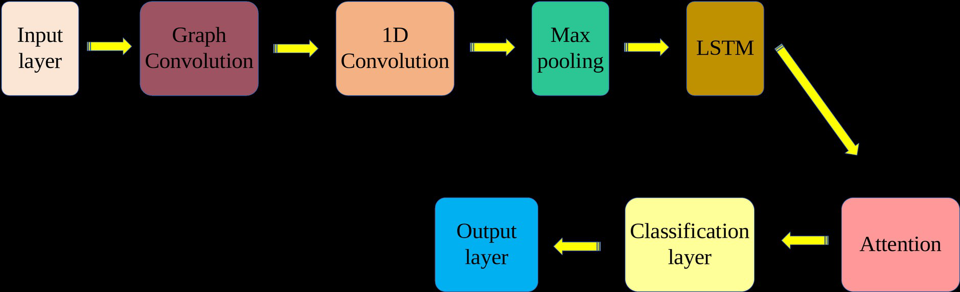
Figure 2: Spatio-Temporal EEGNet
By reducing the dimensionality while maintaining crucial temporal aspects, the Max-Pooling Layer makes sure that the most important data is maintained for classification. The addition of an LSTM layer makes it easier for the model to recognise sequential dependencies in the EEG data. Beyond the receptive field of the preceding layers, it can grasp temporal patterns. An Attention Mechanism operates within the LSTM Layer, enabling the model to concentrate on the most significant time steps for classification. This adaptability makes sure that the model makes the best use of the temporal data. Fully Connected Layers are the next stop on the path, where the spatial and temporal information that were extracted are analysed and one or more fully connected layers with ReLU activation functions offer deeper understanding of the data. The MCO-based Activation Function Optimisation, which tweaks the activation function parameters to increase classification accuracy, is a novel feature of this model. A softmax activation function is also used by the output layer to generate class probabilities for motor imaging tasks. For the purpose of directing the training process, the Classification Loss, which is commonly calculated using the Root Mean Square Error (RMSE), measures the discrepancy between anticipated and actual classes.
4. Result and Discussion
4.1. Experimental setup
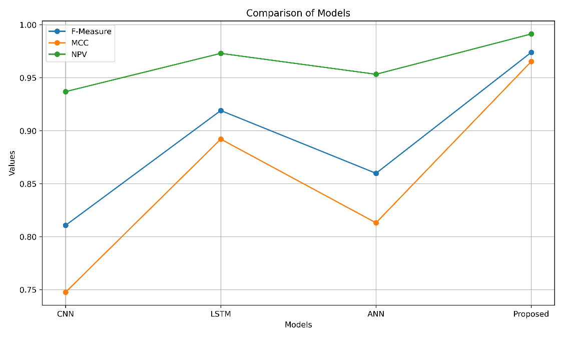
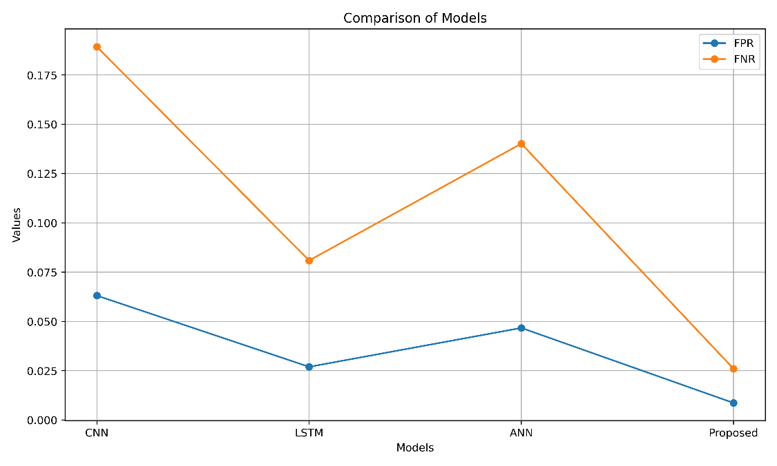
The proposed model is implemented using PYTHON. This work used two datasets, namely Dataset IIa BCI Competition IV [26] and Dataset IVa BCI Competition III [27]. The proposed model is compared with the existing models namely, Convolutional neural network (CNN), long short-term memory (LSTM), Artificial Neural Network (ANN). The performance metrics like accuracy, FNR, FPR, MCC, NPV, precision, sensitivity, specificity, and F-measure are used to evaluate the proposed model.
4.2. Performance Metrics
Accuracy
The percentage of accurately predicted cases to all examples is used to measure accuracy.
Precision
Precision is a helpful indicator of how precisely the positive chemicals are expected because it indicates the percentage of correctly anticipated positive cases to all test findings.
Sensitivity
By dividing the total positives by the percentage of genuine positive forecasts, one may determine the sensitivity number.
Specificity
The percentage of successfully predicted negative outcomes over all negative outcomes is known as specificity.
F_Measure
In order to ensure that each class only contains a single sort of data item, the F-Measure number strikes a compromise between fully identifying all data bits and doing so.
Matthew’s correlation coefficient (MCC)
A binary two-by-two variable association measure is the MCC.
Negative Prediction Value (NPV)
The performance of a diagnostic test or similar quantitative metric is described by NPV.
False Positive Ratio (FPR)
The false positive rate is derived by dividing the total number of negative events by the total number of negative events that were incorrectly labelled as positive (false positives).
False Negative Ratio (FNR)
The “false-negative rate,” sometimes known as the “miss rate,” is the probability that the test will fail to identify a real positive.
4.3. Overall Performance of Proposed Model
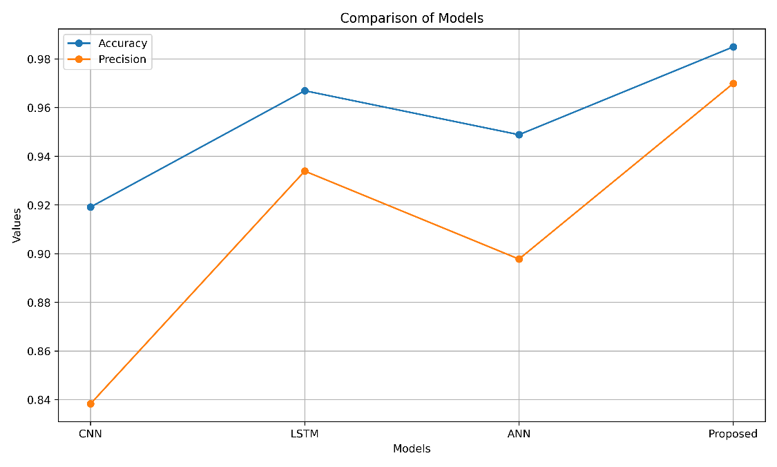
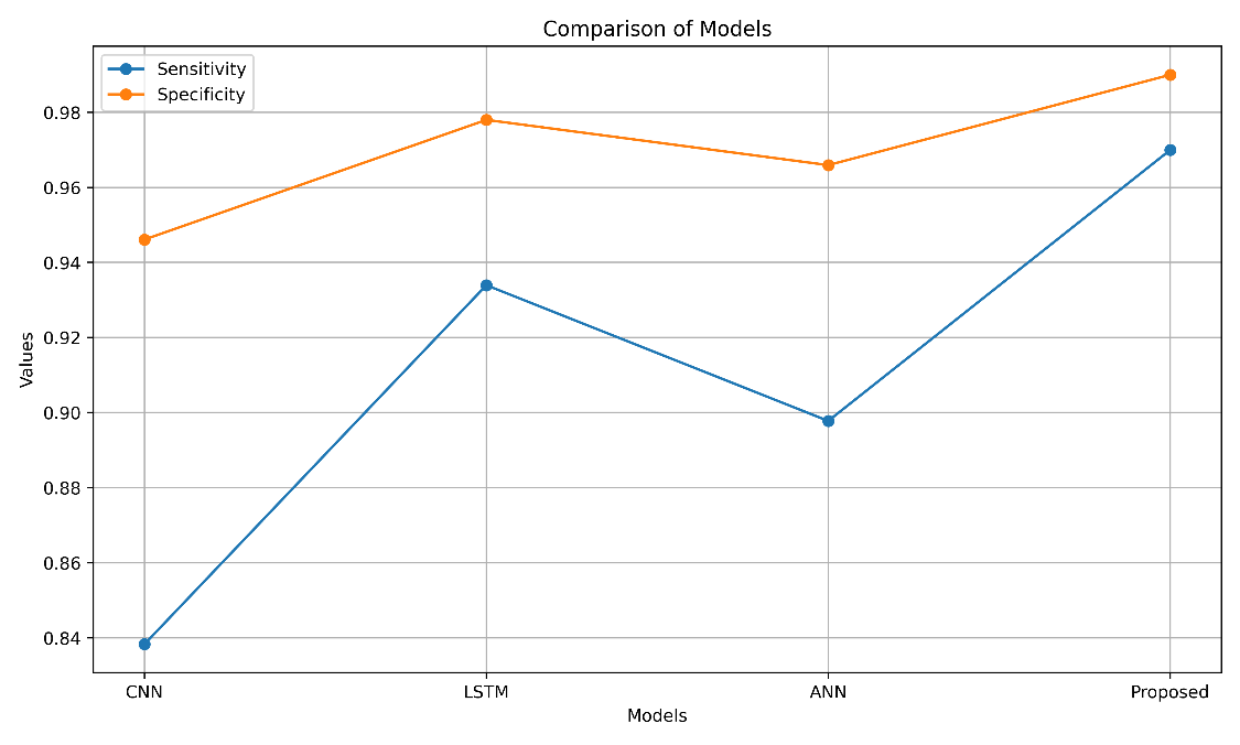
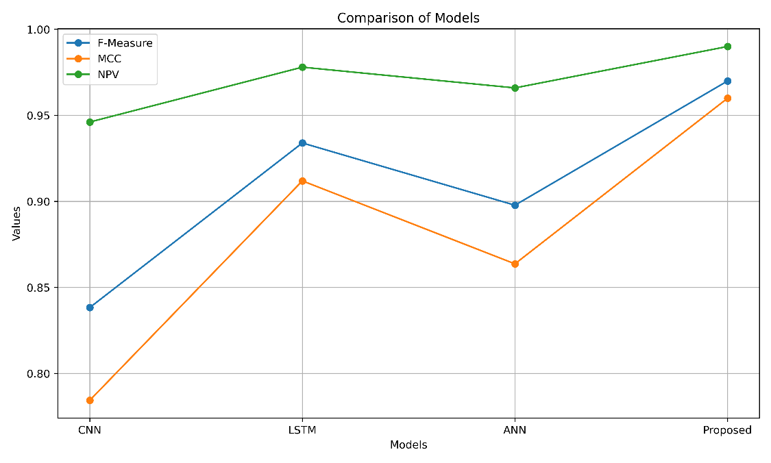
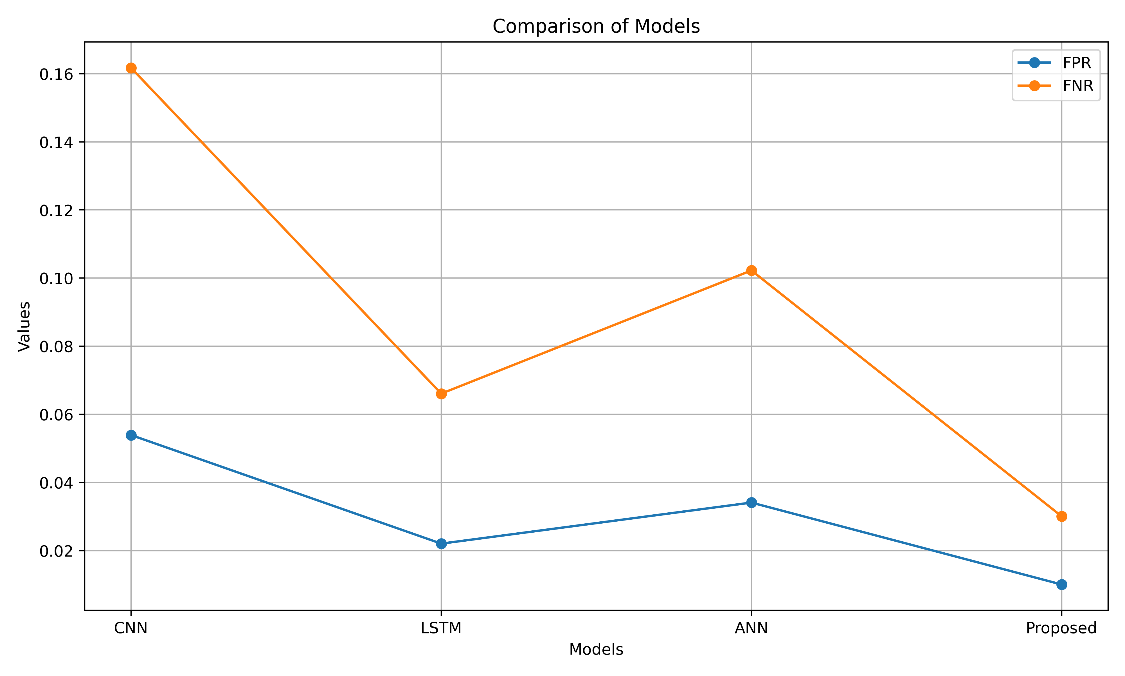
Table 1 provides a comprehensive comparison of different machine learning methods’ performance on Dataset 1. The methods evaluated include CNN, LSTM, ANN, and the proposed model. In terms of accuracy, the proposed model stands out with an impressive score of 98.497%, indicating its ability to make correct predictions with high precision. It outperforms the other methods, where CNN achieves 91.915%, LSTM reaches 96.697%, and ANN attains 94.888%. Precision, which measures the proportion of true positive predictions among all positive predictions, demonstrates the proposed model’s superiority at 96.994%. Sensitivity, representing the true positive rate, also aligns with this high performance, indicating the model’s proficiency in correctly identifying positive cases. Specificity measures the true negative rate, and here too, the proposed model excels at 98.998%, indicating its capability to accurately identify negative cases. The F-Measure, MCC, NPV, FPR, and FNR values further validate the proposed model’s superior performance compared to the other methods. The lower FPR and FNR values indicate a better balance between precision and recall. The proposed model exhibits exceptional performance across various metrics, showcasing its effectiveness in handling Dataset 1 for the classification task.
Table 1: Techniques Comparison – Dataset 1
| Methods | CNN | LSTM | ANN | Proposed |
|---|---|---|---|---|
| Accuracy | 0.919145 | 0.966967 | 0.948883 | 0.98497 |
| Precision | 0.83829 | 0.933933 | 0.897766 | 0.969941 |
| Sensitivity | 0.83829 | 0.933933 | 0.897766 | 0.969941 |
| Specificity | 0.946097 | 0.977978 | 0.965922 | 0.98998 |
| F-Measure | 0.83829 | 0.933933 | 0.897766 | 0.969941 |
| MCC | 0.784386 | 0.911911 | 0.863688 | 0.959921 |
| NPV | 0.946097 | 0.977978 | 0.965922 | 0.98998 |
| FPR | 0.053903 | 0.022022 | 0.034078 | 0.01002 |
| FNR | 0.16171 | 0.066067 | 0.102234 | 0.030059 |
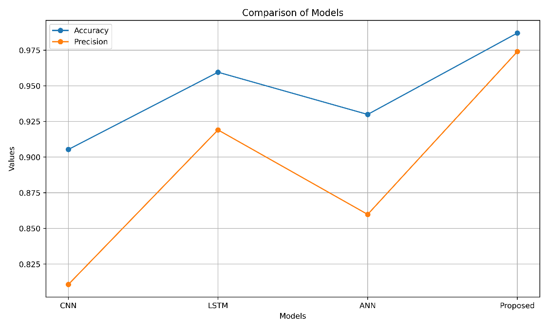
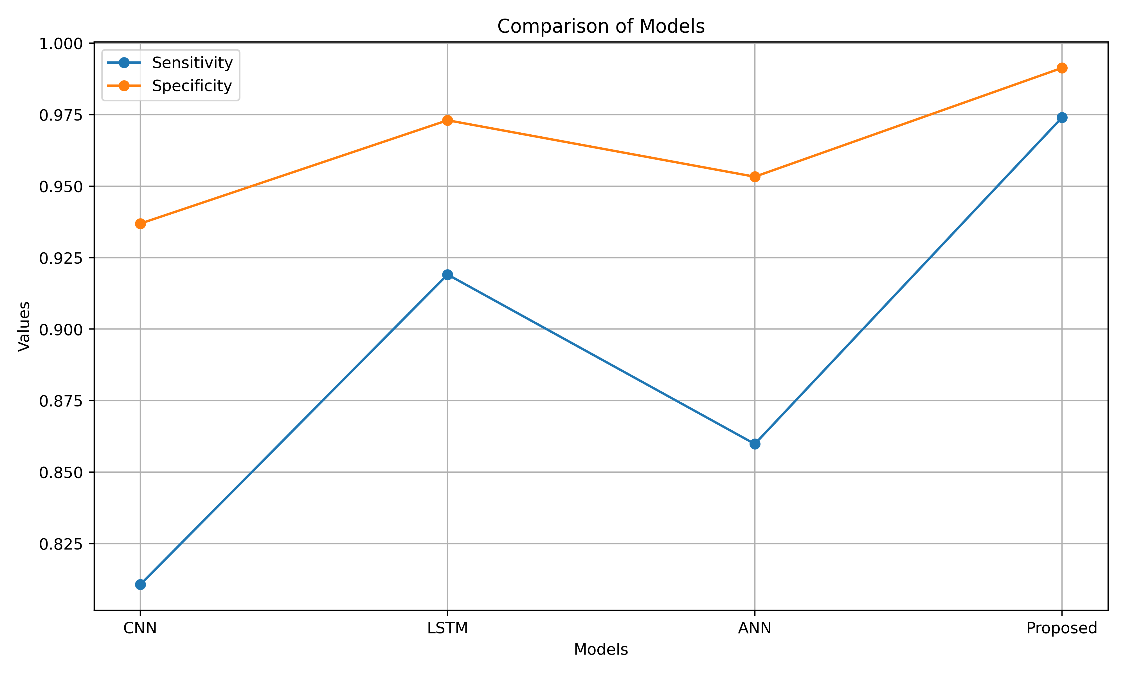
Table 2 provides a comprehensive comparison of the performance metrics for various machine learning methods applied to Dataset 2. the proposed model achieves an outstanding accuracy of 98.699%, indicating that it correctly classifies the vast majority of cases. For the proposed model, it stands at 97.398%, signifying that when it predicts a motor imagery class, it is correct approximately 97.4% of the time. The proposed model achieves a high sensitivity of 97.398%, indicating its proficiency in detecting motor imagery classes when they are present. The proposed model excels with a specificity of 99.133%, signifying its capacity to correctly classify cases as other-class when they are not. The proposed model maintains an F-Measure of 97.398%, demonstrating a balanced trade-off between precision and recall. The proposed model achieves a high MCC of 96.5318%, indicating strong agreement between predicted and actual classifications. The proposed model attains a robust NPV of 99.133%, implying that when it predicts a another motor imagery class, it is correct approximately 99.1% of the time. The proposed model maintains a low FPR of 0.8671%, implying a minimal rate of falsely identifying other motor imagery classes as positive. The proposed model exhibits a low FNR of 2.6012%, indicating a low rate of incorrectly classifying target-class instances as negative. These values collectively demonstrate the superior performance of the proposed model in accurately identifying and classifying motor imagery classes on Dataset 2, with a strong emphasis on both precision and recall, as well as overall accuracy and reliability.
Table 2: Techniques Comparison – Dataset 2
| Methods | CNN | LSTM | ANN | Proposed |
|---|---|---|---|---|
| Accuracy | 0.905347 | 0.959538 | 0.929913 | 0.986994 |
| Precision | 0.810694 | 0.919075 | 0.859827 | 0.973988 |
| Sensitivity | 0.810694 | 0.919075 | 0.859827 | 0.973988 |
| Specificity | 0.936898 | 0.973025 | 0.953276 | 0.991329 |
| F-Measure | 0.810694 | 0.919075 | 0.859827 | 0.973988 |
| MCC | 0.747592 | 0.8921 | 0.813102 | 0.965318 |
| NPV | 0.936898 | 0.973025 | 0.953276 | 0.991329 |
| FPR | 0.063102 | 0.026975 | 0.046724 | 0.008671 |
| FNR | 0.189306 | 0.080925 | 0.140173 | 0.026012 |
Table 3 and Table 4 display the impact of different subjects on the accuracy of Datasets 1 and 2, respectively. Each subject’s influence on the accuracy of the classification model is measured, with varying degrees of impact observed across different subjects in both datasets.
Table 3: Evaluating Subjects: Impact on Datasets1
| Subjects | Accuracy |
|---|---|
| 0 | 0.905582 |
| 1 | 0.902558 |
| 2 | 0.896521 |
| 3 | 0.952661 |
| 4 | 0.865255 |
| 5 | 0.915233 |
| 6 | 0.935471 |
| 7 | 0.941582 |
| 8 | 0.958236 |
Table 4: Evaluating Subjects: Impact on Datasets2
| Subjects | Accuracy |
|---|---|
| 0 | 0.940125 |
| 1 | 0.985621 |
| 2 | 0.859662 |
| 3 | 0.947414 |
| 4 | 0.956214 |
| 5 | 0.945542 |
| 6 | 0.935282 |
| 7 | 0.914524 |
| 8 | 0.914546 |
4.4. Graphical Representation
Fig. 3 presents graphical representations of key performance metrics for Dataset 1. Subplots (a) display accuracy and precision, (b) show sensitivity and specificity, (c) visualize F-Measure, MCC, and NPV, while (d) illustrates FPR and FNR, providing a comprehensive evaluation of the model’s performance.
 |
|---|
| (a) |
 |
| (b) |
 |
| (c) |
 |
| (d) |
Figure 3: Graphical representation for dataset1 (a) accuracy, precision, (b) sensitivity, specificity, (c) f-measure, MCC, NPV, (d) FPR, FNR.
Fig. 4 presents graphical representations of key performance metrics for Dataset 2. Subplots (a) display accuracy and precision, (b) show sensitivity and specificity, (c) visualize F-Measure, MCC, and NPV, while (d) illustrates FPR and FNR, providing a comprehensive evaluation of the model’s performance.
 |
|---|
| (a) |
 |
| (b) |
 |
| (c) |
 |
| (d) |
Figure 4: Graphical representation for dataset2 (a) accuracy, precision, (b) sensitivity, specificity, (c) f-measure, MCC, NPV, (d) FPR, FNR.
 |  |
|---|---|
| (a) | (b) |
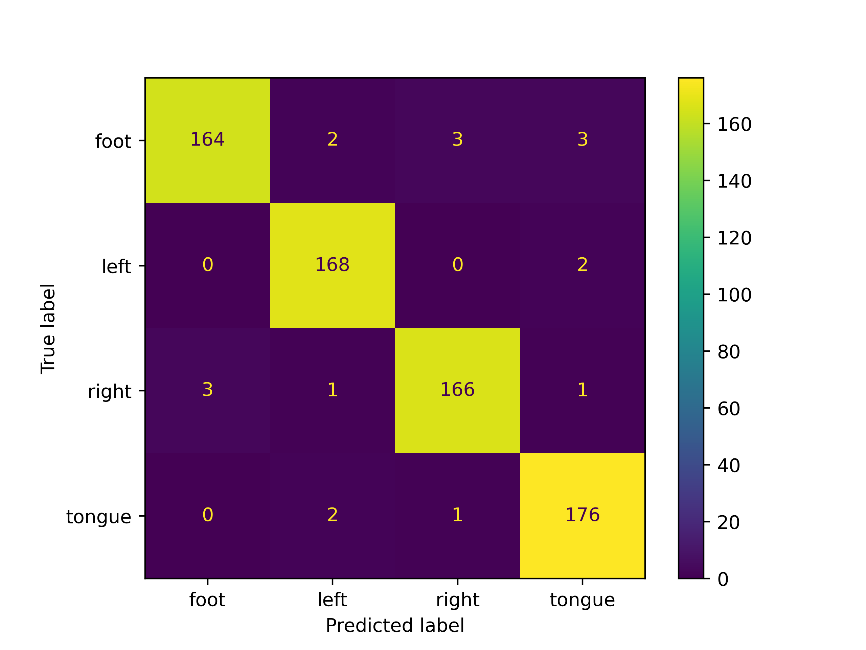
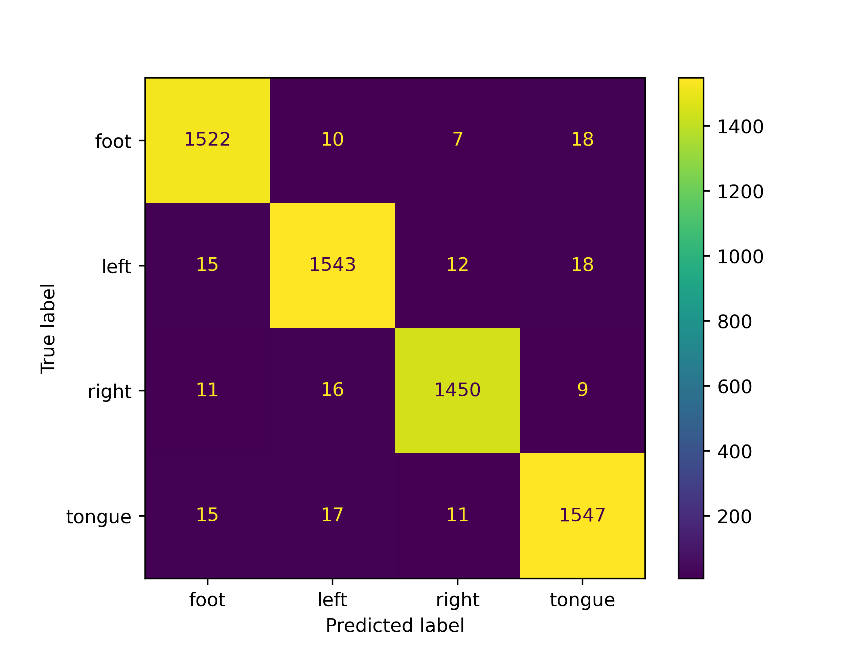
Figure 5: Confusion matrix (a) dataset1 (b) dataset2
Fig. 5 displays the confusion matrices for dataset1 (a) and dataset2 (b). These matrices summarize the performance of a classification model, indicating the counts of true positives, true negatives, false positives, and false negatives for each dataset.
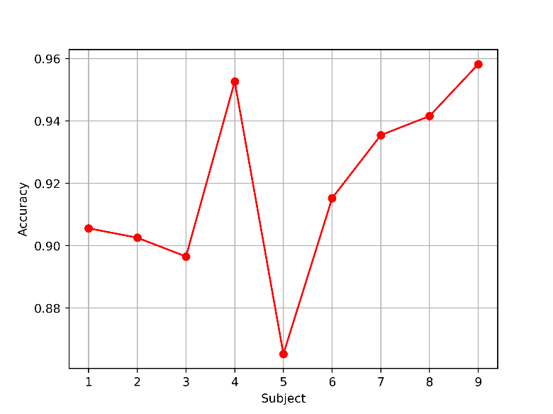
Figure 6: Subjects accuracy – dataset1
Fig. 6 and Fig. 7 illustrate the accuracy of different subjects in dataset1 and dataset2, showcasing variations in individual subject performance.
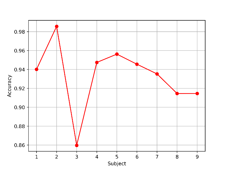
Figure 7: Subjects accuracy – dataset2
5. Conclusion
This work introduced a novel method that improved the effectiveness and precision of BCI systems based on EEG data. The suggested methodology had six essential steps. SMOTE was used in data augmentation to enrich the dataset and increase its representativeness. To capture underlying oscillatory components, EMD was first introduced in signal pre-processing along with notch filtering, ICA, time windows, and other techniques. The new MCO model, a combination of the MFO and COA, was introduced through optimal channel selection. A variety of features, including time-domain properties, frequency-domain attributes, connectivity measures, and IMFs-based features that capture oscillatory patterns, were extracted from the chosen EEG channels and IMF. To improve the feature selection process and strike a balance between exploration and exploitation, Feature Selection created the hybrid optimisation model MCO. The creation of the Spatio-Temporal EEGNet, a personalised deep learning model, was required for classification via this method. Python was used to put the proposed model into practise.
Reference
Jin, J., Liu, C., Daly, I., Miao, Y., Li, S., Wang, X. and Cichocki, A., 2020. Bispectrum-based channel selection for motor imagery-based brain-computer interfacing. IEEE Transactions on Neural Systems and Rehabilitation Engineering, 28(10), pp.2153-2163.
Varsehi, H. and Firoozabadi, S.M.P., 2021. An EEG channel selection method for motor imagery-based brain–computer interface and neurofeedback using Granger causality. Neural Networks, 133, pp.193-206.
Chen, J., Yu, Z., Gu, Z. and Li, Y., 2020. Deep temporal-spatial feature learning for motor imagery-based brain–computer interfaces. IEEE Transactions on Neural Systems and Rehabilitation Engineering, 28(11), pp.2356-2366.
Huang, Z. and Wei, Q., 2023. Tensor decomposition-based channel selection for motor imagery-based brain-computer interfaces. Cognitive Neurodynamics, pp.1-16.
Ren, S., Wang, W., Hou, Z.G., Liang, X., Wang, J. and Shi, W., 2020. Enhanced motor imagery-based brain-computer interface via FES and VR for lower limbs. IEEE Transactions on Neural Systems and Rehabilitation Engineering, 28(8), pp.1846-1855.
Fumanal-Idocin, J., Wang, Y.K., Lin, C.T., Fernández, J., Sanz, J.A. and Bustince, H., 2021. Motor-imagery-based brain–computer interface using signal derivation and aggregation functions. IEEE Transactions on Cybernetics, 52(8), pp.7944-7955.
Jin, J., Sun, H., Daly, I., Li, S., Liu, C., Wang, X. and Cichocki, A., 2021. A novel classification framework using the graph representations of electroencephalogram for motor imagery-based brain-computer interface. IEEE Transactions on Neural Systems and Rehabilitation Engineering, 30, pp.20-29.
Zhang, S., Zhu, Z., Zhang, B., Feng, B., Yu, T. and Li, Z., 2020. Fused group lasso: A new EEG classification model with spatial smooth constraint for motor imagery-based brain–computer interface. IEEE Sensors Journal, 21(2), pp.1764-1778.
Sun, B., Wu, Z., Hu, Y. and Li, T., 2022. Golden subject is everyone: A subject transfer neural network for motor imagery-based brain computer interfaces. Neural Networks, 151, pp.111-120.
Abenna, S., Nahid, M. and Bajit, A., 2022. Motor imagery-based brain-computer interface: improving the EEG classification using Delta rhythm and LightGBM algorithm. Biomedical Signal Processing and Control, 71, p.103102.
Parashiva, P.K. and Vinod, A.P., 2022. Improving direction decoding accuracy during online motor imagery-based brain-computer interface using error-related potentials. Biomedical Signal Processing and Control, 74, p.103515.
Zheng, M., Yang, B., Gao, S. and Meng, X., 2021. Spatio-time-frequency joint sparse optimization with transfer learning in motor imagery-based brain-computer interface system. Biomedical Signal Processing and Control, 68, p.102702.
Mashat, M.E.M., Lin, C.T. and Zhang, D., 2019. Effects of task complexity on motor imagery-based brain–computer interface. IEEE Transactions on Neural Systems and Rehabilitation Engineering, 27(10), pp.2178-2185.
Xia, K., Deng, L., Duch, W. and Wu, D., 2022. Privacy-preserving domain adaptation for motor imagery-based brain-computer interfaces. IEEE Transactions on Biomedical Engineering, 69(11), pp.3365-3376.
Pillette, L., Roc, A., N’kaoua, B. and Lotte, F., 2021. Experimenters’ influence on mental-imagery based brain-computer interface user training. International Journal of Human-Computer Studies, 149, p.102603.
Ko, L.W., Lu, Y.C., Bustince, H., Chang, Y.C., Chang, Y., Ferandez, J., Wang, Y.K., Sanz, J.A., Dimuro, G.P. and Lin, C.T., 2019. Multimodal fuzzy fusion for enhancing the motor-imagery-based brain computer interface. IEEE Computational Intelligence Magazine, 14(1), pp.96-106.
Deng, X., Zhang, B., Yu, N., Liu, K. and Sun, K., 2021. Advanced TSGL-EEGNet for motor imagery EEG-based brain-computer interfaces. IEEE access, 9, pp.25118-25130.
Fumanal-Idocin, J., Takáč, Z., Fernández, J., Sanz, J.A., Goyena, H., Lin, C.T., Wang, Y.K. and Bustince, H., 2021. Interval-Valued Aggregation Functions Based on Moderate Deviations Applied to Motor-Imagery-Based Brain–Computer Interface. IEEE Transactions on Fuzzy Systems, 30(7), pp.2706-2720.
Lazurenko, D.M., Kiroy, V.N., Shepelev, I.E. and Podladchikova, L.N., 2019. Motor imagery-based brain-computer interface: neural network approach. Optical Memory and Neural Networks, 28, pp.109-117.
Zhang, S., Wang, S., Zheng, D., Zhu, K. and Dai, M., 2019. A novel pattern with high-level commands for encoding motor imagery-based brain computer interface. Pattern Recognition Letters, 125, pp.28-34.
Shi, B., Wang, Q., Yin, S., Yue, Z., Huai, Y. and Wang, J., 2021. A binary harmony search algorithm as channel selection method for motor imagery-based BCI. Neurocomputing, 443, pp.12-25.
Sun, B., Liu, Z., Wu, Z., Mu, C. and Li, T., 2022. Graph convolution neural network based end-to-end channel selection and classification for motor imagery brain-computer interfaces. IEEE transactions on industrial informatics.
Zuo, C., Miao, Y., Wang, X., Wu, L. and Jin, J., 2020. Temporal frequency joint sparse optimization and fuzzy fusion for motor imagery-based brain-computer interfaces. Journal of Neuroscience Methods, 340, p.108725.
Moumgiakmas, S.S. and Papakostas, G.A., 2022. Robustly effective approaches on motor imagery-based brain computer interfaces. Computers, 11(5), p.61.
Togha, M.M., Salehi, M.R. and Abiri, E., 2019. Improving the performance of the motor imagery-based brain-computer interfaces using local activities estimation. Biomedical Signal Processing and Control, 50, pp.52-61.
Dataset1 collected from: “https://www.bbci.de/competition/iv/”, dated 01-06-2023.
Dataset2 collected from: “https://www.bbci.de/competition/iii/desc_IVa.html”, dated 01-06-2023.
Cite This Work
To export a reference to this article please select a referencing stye below:

Academic Master Education Team is a group of academic editors and subject specialists responsible for producing structured, research-backed essays across multiple disciplines. Each article is developed following Academic Master’s Editorial Policy and supported by credible academic references. The team ensures clarity, citation accuracy, and adherence to ethical academic writing standards
Content reviewed under Academic Master Editorial Policy.





