
Abstract
Speech enhancement aims to recover useful voice information from noise-corrupted signals. IntelliNoiseFilter combines dataset preparation, feature extraction, ConvRecGRU-based noise estimation, OptiKalFilter-based noise filtering and evaluation. The preparation stage adds additive white Gaussian noise (AWGN) to the input signals. Mel-spectrum, spectral chroma, Mel-frequency cepstral coefficients and Gammatone features represent complementary signal characteristics. ConvRecGRU combines convolutional, recurrent and gated recurrent neural-network components, with a hybrid Cat Swarm Optimization and Anarchic Society Optimization procedure. OptiKalFilter applies optimized Kalman filtering to reduce residual noise. The supplied MATLAB evaluation compares the proposed model with CNN, RNN, GRU, Bi-LSTM and LSTM baselines and reports an accuracy of 0.967. The classification results and their scope are discussed separately from perceptual speech-quality evaluation.
Keywords: IntelliNoiseFilter, Speech enhancement, ConvRecGRU, OptiKalFilter, Anarchic Society Optimisation and Cat Swarm Optimisation
Introduction
Speech is a natural form of human communication, but recorded signals frequently contain environmental noise. Speech enhancement is therefore an important component of digital speech processing. Its objectives include reducing background noise, improving perceived quality and retaining intelligibility. An effective enhancement method must balance noise suppression against distortion of useful speech information. This balance is relevant to communication systems, recognition applications and assistive listening devices.
Speech-enhancement systems can be categorized by the number of microphones they use. Single-channel methods process one microphone signal, while multichannel methods exploit several spatially separated observations. Although additional channels can provide useful spatial information, single-channel enhancement remains relevant where hardware, cost or deployment constraints limit the available inputs. Spectral subtraction, Wiener filtering and minimum mean-square-error estimation are established approaches, while learning-based methods seek to model more complex relationships between noisy inputs and useful signal components.
Deep learning has expanded the range of data-driven approaches to speech enhancement. Unlike methods based primarily on fixed statistical assumptions, neural networks learn representations and mappings from training examples. Their performance depends on the data, noise conditions and evaluation protocol, so improvement is not automatic in every setting. Hybrid designs combine learned features with structured signal-processing methods. This work follows that direction by combining neural noise estimation with Kalman filtering. The related literature and the proposed processing stages are presented below.
For related implementation constraints, low-latency FIR signal processing discusses filter hardware costs. Those circuit-level concerns are distinct from the model evaluation reported here.
Literature Review
Shimada, K., et al [1] have suggested utilising effective initialization and incremental MNMF parameter updating to implement online minimum variance distortionless response (MVDR) beamforming. Another significant addition was the thorough analysis of the ASR performances produced by different spatial filter types, including rank-1 and full-rank multichannel Wiener filters, time-invariant and variant MVDR beamformers, and others, when used in conjunction with MNMF.
Sadeghi, M., et al [2] have presented Variational auto-encoders (VAE) for single-channel and speaker-independent speech improvement. In order to condition the audio speech generation process on visual input of the lip region, a conditional VAE (CVAE) was created. Speech enhancement utilised a Monte Carlo expectation maximisation approach, and the audio-visual speech generating model was merged with a noise framework that utilised nonnegative matrix factorization during testing.
Garg, A. and Sahu, O.P., [3] have provided a hybrid approach to reduce the signal’s noise. First, the database’s robust signal was retrieved, and it was then pre-reconstructed with the use of empirical mode decomposition. The resulting reconstructed signal was then used as the input of the Bionic Wavelet Transform (BWT), which produced the de-noised signal. The denoised signal was adjusted using a Butterworth filter. In order to derive the final de-noised signal, inverse BWT was used. The MATLAB platform used the suggested methods.
Srinivasarao, V. and Ghanekar, U., [4] have applied a modified Kalman filter to remove noise from speech samples. To improve speech clarity and quality, a Kalman filter built using Principal Component Analysis (PCA) was suggested. The simulation results demonstrated superior performance than Wiener filter, Modulation Compressive Sensing, Compressed Sensing Frequency, and Log Minimum Mean Square Error (LogMMSE), proving the effectiveness of the suggested technique for augmenting speech signals.
Yu, H., et al [5] have suggested a hybrid speech improvement system with the goal of enhancing performance in the presence of unknown noise. This system used deep neural networks (DNN) for voice reconstruction and Kalman filtering for further denoising. First, two distinct DNNs were trained to learn the mapping from noisy acoustic data to the clean speech magnitudes and line spectrum frequencies (LSFs), correspondingly. The estimated clean speech was then recreated by fusing the estimated clean magnitudes with the noisy speech’s phase, and Kalman filtering was applied by converting the LSFs to linear prediction coefficients (LPCs). The residual noises were further eliminated by applying a Kalman filter to the reconstructed speech.
Dash, T.K. and Solanki, S.S., [6] have developed a brand-new hybrid paradigm for improving speech. The creation of clean speech spectrograms with excellent intelligibility was described by the proposed system as a difficult challenge, and the success of the proposed method was confirmed. The MATLAB platform was used for the implementation. The experimental findings demonstrated that the suggested technique produced superior outcomes with higher PESQ, higher SNR, and lower MMSE.
Gnanamanickam, J., et al [7] have utilized a hybridised algorithm to improve the accuracy of speech recognition. They suggested combining the Hidden Markov Model with the well-known non-linear spectral subtraction speech enhancement technique for optimum performance. The suggested approach was tested using 1440 Ryerson Audio-Visual Database of Emotional Speech and Song (RAVDESS) audio files and 6660 medical speech transcription audio files. A number of common speech enhancement strategies, including the iterative signal enhancement algorithm, subspace-based speech enhancement, and non-linear spectral subtraction, were used to compare the performance of the suggested model.
Yu, H., et al [8] have developed a new colored-noise Kalman filter-based deep neural network (DNN)-augmented speech enhancement system. In their approach, driving noise variances and linear prediction coefficients (LPCs) were used as parameters to describe both clean speech and noise as autoregressive (AR) processes. While the driving noise variances were acquired by solving an optimisation problem to reduce the discrepancy between the modelled and observed AR spectra of the noisy speech, the LPCs were acquired by training a multi-objective DNN that learned the mapping from the noisy acoustic features to the line spectrum frequencies (LSFs). The noisy speech was then subjected to the colored-noise Kalman filter with DNN calculated parameters for denoising. Finally, a post-subtraction technique was used to further reduce the noise in the speech that had been Kalman filtered.
Mahmmod, B.M., et al [9] have focused on using models that match well with speech and noisy data signals to derive the best low-distortion estimator. First, the observation signal was transformed into a transform domain using a recent transform based on an orthogonal polynomial. To create precise and flexible models for noise signals, feature extraction-based noise classification was used. Thirdly, two steps of nonlinear and linear estimators utilising the least mean square error (MMSE) and novel models for speech and noise were developed to estimate a clean speech signal. Finally, the inverse of the orthogonal transform was taken into account to determine the predicted speech signal in the time domain.
Park, G., et al [10] have used noise reduction strategies with deep neural network learning utilising noise categorization to present a voice enhancement algorithm to increase speech quality in a hearing aid setting. Convolutional neural networks were used to self-record and categorise 10 different types of noise in order to test speech improvement in a real hearing aid setting. Deep neural networks based on the noise categorization were then used to provide noise reduction for speech enhancement in the hearing aid.
Proposed methodology
The proposed pipeline processes noise-corrupted signals through preparation, feature extraction, noise estimation, filtering and evaluation. AWGN is introduced during preparation. Mel-spectrum, spectral chroma, MFCC and Gammatone features describe complementary spectral characteristics. ConvRecGRU combines optimized CNN components with RNN and GRU components to estimate noise. A hybrid of Cat Swarm Optimization and Anarchic Society Optimization supplies the optimization procedure. OptiKalFilter then applies optimized Kalman filtering. Figure 1 summarizes the supplied workflow.
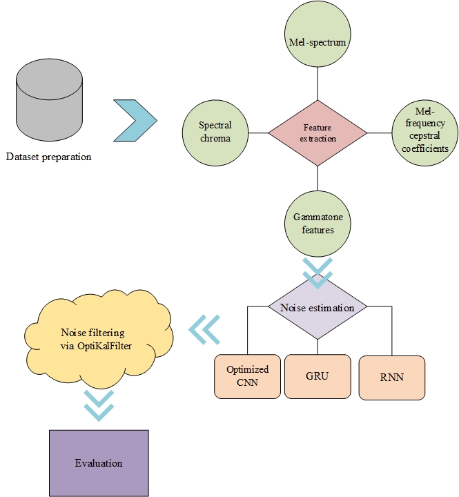
Figure 1. Overall proposed work
3.1 Dataset preparation
Additive white Gaussian noise is added to the input signal sample by sample. Its amplitude follows a Gaussian distribution centered on zero mean and a chosen standard deviation. The standard deviation controls the noise power. The term white refers to a flat power spectral density, while additive means that the noise is combined with the signal by addition.
To construct the noisy input, random samples are drawn from the specified Gaussian distribution and added to the corresponding clean-signal samples. AWGN is convenient for analytical modeling and controlled experiments. It does not represent every environmental noise condition, however, so results obtained with this model should be interpreted within the conditions of the supplied evaluation.
3.2 Feature extraction
The speech signals are processed to extract different features. Among these features is the Mel-spectrum, which highlights perceptually significant frequency bands by computing the Mel-scale power spectrogram. The distribution of chroma or pitch classes in the audio stream is represented by the chromagram, which is calculated by the spectral chroma. The contour of the power spectrum in the Mel-frequency domain is captured through the extraction of the Mel-frequency cepstral coefficients (MFCC). A filterbank that simulates auditory perception based on the human auditory system is also used to extract gamma-tone features.
Mel-spectrum
The Mel-spectrum is a representation of the speech signal based on the Mel scale that highlights perceptually significant frequency regions. An approximation of the non-linear frequency resolution of the human auditory system, the Mel scale is a perceptual scale of pitches. A spectrogram is a graphic representation of the frequency spectrum of a signal over time. The following formula, where m stands for Mels and f for Hertz, relates the Mel scale to Hertz and offers a linear scale for the human auditory system:
\(m = 2595\log_{10}\ (1 + \frac{f}{700})\)
The Mel spectrogram is employed to give our models sound data similar to what a human would hear. The Mel spectrogram is produced by running the raw audio waveforms through filter banks. Each sample now has a form of 128 x 128 (corresponding to 128 filter banks and 128-time steps per clip), showing that this procedure was employed.
Mel-frequency cepstral coefficients (MFCC)
Mel-frequency cepstral coefficients (MFCCs) are a popular feature representation in speech recognition and audio signal processing. They give a condensed representation of the spectral content of a signal and are produced from its power spectrum. Extract the coefficients that capture the shape of the power spectrum in the Mel-frequency domain. The MFCC is the most popular feature extraction. This aids in characterising the speech signal characteristics. For speech recognition, the MFCC is found to be better, and it helps in creating human perception compassion which takes into account the frequencies. The computation for Mel log energies based on discrete cosine transform (DCT) is carried out in the MFCC extraction methods.
Framing
The signal is divided into frames of N samples with a frame advance of M samples, where 0 < M < N for overlapping frames. The first frame contains the initial N samples, and each subsequent frame starts M samples later. Adjacent frames therefore overlap by N − M samples. The process continues until the signal has been covered.
Windowing
This aids in reducing the signal’s discontinuity at the beginning and the end of each frame. The windowing procedure is primarily designed to reduce the signal’s spectral distortion. At the start of each frame and at its end, the signal is reset to zero.
\(S(x),\ \ \ \ \ \ \ \ \ \ \ \ 0 \leq x \leq N – 1\)
Here, N is the number of samples in a frame, and x indexes the samples within that frame.
Fast Fourier Transform
The fast Fourier transform converts each windowed frame from the time domain to a frequency-domain representation. The complex-valued coefficients describe magnitude and phase. Their magnitudes provide spectral information for subsequent filterbank processing.
\(Y_{N} = \ \left\{ \begin{array}{r} 0 < F < \frac{F^{s}}{2}\ \ \ \ \ \ \ \ \ \ positive\ frequency\ \\ \frac{F^{s}}{2} < F < 0\ \ \ \ \ \ \ \ \ negative\ frequency\ \end{array} \right.\ \ \ \ \ \ related\ to\ \ 0 \leq x \leq \frac{N}{2} – 1\)
The sampling frequency is denoted by Fs. The frequency-domain representation supplies the spectrum or periodogram used in subsequent analysis.
Mel frequency warping and log
Scale values in a speech signal that are linear can be followed by using Mel-frequency warping. Different frequencies can be heard in the sound of human sensitivity. Not all frequencies are found on a linear scale. The real frequency for each tone in the transmission through Hz is determined. On a scale known as the Mel scale, the pitch associated with the tone is provided. Logarithmic spacing will be above 1000 Hz on the Mel frequency scale, while linear frequency spacing will be below 1000 Hz.
DCT
The final MFCC stage applies a discrete cosine transform (DCT) to the log Mel-filterbank energies. The resulting cepstral coefficients provide a compact representation of the spectral envelope. In the expression below, K is the number of filterbank energies, k indexes those energies, and N indexes the retained coefficient.
\({MF}_{N}\ = \ \sum_{k = 1}^{K}\left( \log M_{k} \right)\ \cos\left\lbrack N\left( k – \ \frac{1}{2} \right)\ \frac{\pi}{K} \right\rbrack\ \ \ N = 0,1,\ldots.K – 1\)
The input signal’s mean parameter is represented by the initial component.
Gammatone features
Gammatone features are a frequent feature representation type in audio signal processing, particularly in tasks involving speech recognition and modelling of auditory perception. They are created using a filterbank that simulates the human hearing system’s frequency selectivity. The purpose of the Gammatone filters is to mimic the functioning of the human auditory system. Under this definition, a gamma-tone filter with frequency \(f_{c}\) is:
\(G(t) = at^{k – 1}e^{- 2\pi bt}\cos\left( 2\pi f_{c}t + \varphi \right)\)
where \(k\) determines the order of the filter and is often set to a value less than 4, the constant \(a\) controls the gain, and \(\varphi\) is the phase but is typically set to zero. The following is the factor b:
\(b = 25.17\ \left( \frac{4.37\ f_{c}}{1000}\ + 1\ \right)\)
A collection of Gammatone filters, also known as channels with various centre frequencies, are used to build a Gammatone filter-bank in order to produce a representation that resembles an FFT-based spectrogram. Each of the gammatone filters is convolved with the input audio signal to produce the filterbank response. Convolution captures the spectral information of the signal inside the filter’s frequency range by computing the filter’s response at each instant in time. Each filter in the bank goes through this procedure, producing a set of filterbank outputs in the process.
3.3 Noise Estimation
ConvRecGRU combines convolutional neural networks, recurrent neural networks and gated recurrent units for noise estimation. The model is trained to estimate noise from the input features. The supplied optimization procedure combines Cat Swarm Optimization and Anarchic Society Optimization to tune the CNN component.
Cat Swarm Optimization
Hybrid search procedures are also used in cat-swarm-based wireless sensor routing. That application has a different objective; here the search is applied to the supplied noise-estimation pipeline.
Cat Swarm Optimization (CSO) represents candidate solutions as cats in an M-dimensional search space. Its seeking mode explores nearby candidate positions, while its tracing mode updates positions through velocities directed by the search history. A mixture ratio controls the balance between these modes. The following steps describe the supplied hybrid procedure.
Step 1: Initialization
Set the population size \(m\), maximum iteration \(\max_{iter}\), mixture ratio (\(MR\)), and randomly initialise position of the cat population between \(\lbrack a\ b\rbrack\); this is represented with the row vector \(Y\) to start the cat swarm.
Step 2: Generate Oppositional solutions
The tent map’s expression for individual location updates is as follows:
\(x_{i}^{\max_{iter} + 1} = \ \ \left\{ \begin{array}{r} 2x_{i}^{\max_{iter}},\ \ \ \ \ \ \ \ \ \ \ \ \ \ \ \ \ \ \ \ 0 \leq \ x_{i}^{\max_{iter}} \leq 0.5 \\ 2\left( 1 – \ x_{i}^{\max_{iter}} \right),\ \ \ \ \ \ \ \ \ \ \ \ 0.5 \leq \ x_{i}^{\max_{iter}} \leq 1\ \ \ \ \end{array} \right.\ \)
Where \(x_{i}^{\max_{iter}}\ \epsilon\ \lbrack 0,1\rbrack,\ i = 1,2,\ldots\ldots.m\). \(\max_{iter} = 1,2,\ldots\ldots.\overline{\max_{iter}}\). \(x_{i}^{\max_{iter}}\ \epsilon\ \lbrack 0,1\rbrack\) can be mutually mapped transformation with the chaotic variables \(Y_{i}^{\max_{iter}}\ \epsilon\ \lbrack a\ b\rbrack\) through
\(x_{i}^{\max_{iter}} = \ \frac{\left( Y_{i}^{\max_{iter}} – a \right)}{(b – a)}\)
\(Y_{i}^{\max_{iter}} = a + \ \ x_{i}^{\max_{iter}}\ (b – a)\)
Step 3: Fitness Computation
Evaluate the fitness of each cat and retain the best candidate according to the minimization objective.
\(Fit = min(E)\)
Step 4: Group the cats based on MR
Assign cats to seeking and tracing groups using the mixture ratio MR, chosen in the interval [0, 1]. A small MR places most cats in seeking mode and a smaller proportion in tracing mode.
Step 5: Classify the cats
Determine the assigned mode for each cat. Apply the seeking procedure to cats in seeking mode and the tracing procedure to cats in tracing mode.
Proposed Seeking Mode
Seeking mode explores candidate positions near the current solution. Copies of a cat’s position are modified, evaluated and compared. The seeking memory pool (SMP) controls the number of candidates, the seeking range of the selected dimension (SRD) controls the perturbation range, the count of dimensions to change (CDC) controls the dimensions modified, and self-position consideration (SPC) determines whether the unchanged position is included.
Following is an explanation of the seeking mode’s operation.
Step 1: Make j copies of \({cat}_{i}\) current position, with \(x\) equaling SMP. Let \(x\) = (SMP-1) if SPC has a true value, and if so, keep the current position as one of the candidates.
Step 2: Replace the previous values for each copy with new ones that are randomly plus or minus SRD percents of the current values, as recommended by CDC.
\({Xjd}_{new\ } = {Xjd}_{old\ }\ (1 + Gauss\left( {Xjd}_{old\ },\tau \right)) + \ {Xjd}_{rand} – r_{1}SRD\left| {Xjd}_{rand} – 2r_{2}{Xjd}_{old\ } \right|\)
where \(j\) is the number of a cat, \(d\) is the dimensions, \({Xjd}_{old\ }\) is the current position, \({Xjd}_{new\ }\) is the next position, and \(rand\) is a random number in the range [0, 1].
\(Gauss\left( {Xjd}_{old\ },\tau \right)\) – Gaussian distribution centered on \({Xjd}_{old\ }\)
\(\tau\) – Standard deviation
\({Xjd}_{old\ }\)– Current position of the solution
\({Xjd}_{new\ }\)– Next position of the solution
\(r_{1},r_{2}\)– random numbers [0 1].
Step 3: Compute each candidate point’s fitness values \((Fit)\).
Step 4: Compute the selection probability using the expression below when candidate fitness values differ. If all candidate fitness values are equal, use equal selection probabilities.
Step 5: Replace the position of \({cat}_{i}\) by selecting a random point from the candidate points.
\(P_{y} = \ \frac{\left| {Fit}_{y} – \ {Fit}_{b} \right|}{{Fit}_{\max} – \ {Fit}_{\min}}\) , where \(0\ < y < x\)
If finding the smallest solution is the fitness function’s aim, then \(\ {Fit}_{b} = {Fit}_{\max}\) ; otherwise, \({Fit}_{b} = \ {Fit}_{\min}\).
Proposed Tracing Mode
Tracing mode updates a cat’s velocity and position using the current search state. Each dimension has an initial velocity, and subsequent iterations apply the velocity update below.
Step 1: Update the velocity in each dimension using the following expression.
Step 2: If a velocity exceeds the specified limit, clip it to the maximum permitted magnitude.
Step 3: Update the cat’s position using the position-update expression given below.
\(v_{j.d} = \ W.v_{j.d} + \ r_{1}\ \times \ \beta_{1}\ \times \left( {Xjd}_{best\ }–\ {Xjd}_{rand\ } \right) + \ \alpha*EI(t)\ \)
\(\beta_{1}\ \) – acceleration coefficient
\(W\) – Inertia weight
\({Xjd}_{best\ }\) – Global best position of solution
Where \(\alpha = \ \alpha_{\max} – \ \left\{ \frac{\alpha_{\max} – \ \alpha_{\min}}{t_{\max}} \right\}*FI(t)\)
\(\alpha_{\max}\) – upper limit of control parameter \(\alpha\)
\(\alpha_{\min}\) – lower limit of control parameter \(\alpha\)
\(t\) – current iteration
\(\beta(t) = \ \beta_{\min} + \left( \beta_{\max} – \ \beta_{\min} \right)\sin\left( \frac{\pi t}{t_{\max}} \right)\)
\(\beta(t)\) is the parameter that influences the global exploration ability.
\(FI(t)\) is the fickleness index, where,
\({FI}_{i}(k) = 1 – \ \alpha_{i}\frac{l\left( A^{*}(k) \right)}{l\left( A_{i}(k) \right)} – (1 – \alpha_{i})\frac{l\left( P_{i}(k) \right)}{l\left( A_{i}(k) \right)}\)
\({FI}_{i}(k) = 1 – \ \alpha_{i}\frac{l\left( G(k) \right)}{l\left( A_{i}(k) \right)} – (1 – \alpha_{i})\frac{l\left( P_{i}(k) \right)}{l\left( A_{i}(k) \right)}\)
\(EI(t)\) is the External Irregularity index.
(c) Information exchange process
The near-best solutions might have changed during the information-exchange process and been transferred into various groups. There are three steps to this process:
For each group, arrange the virtual cats according to their fitness scores.
Replace the worst candidate in each group with a candidate selected from another group. Candidate ranking must follow the chosen minimization objective.
Follow step 2 again for each group.
Step 6: Save the best solution.
Step 7: Return the best solution \({Xjd}_{best\ }\).
Step 8: Terminate.
The best retained solution supplies the reference position for subsequent updates. Random coefficients control stochastic exploration.
\(X_{k,dnew} = \ X_{k,dold} + \ v_{k.d}\)
Here, Xk,dold is the current position of cat k in dimension d, and Xk,dnew is its updated position.
When these two modes are combined, CSO is able to advance towards the global solution in the M-dimensional solution space. The quantity of cats in the tracing subgroup should be low since they spend too little time in this mode. The mixing ratio (MR), which has a modest value, is used to define this quantity. The cat with the best solution will be saved in the memory once the cats have been divided into these two modes, which will result in new locations and fitness functions. Repeat these actions until the termination criteria are met.
The CSO’s computational processes can be summarised as follows:
Step 1: In the process, generate N cats.
Step 2: Sprinkle the cats at random over the M-dimensional solution space, and then choose at random values for each cat’s velocity that fall within the range of the maximum velocity. Select a random number of cats, put some of them in seeking mode according to MR (mixture ratio), and put the others in tracing mode.
Step 3: Apply the positions of the cats to the fitness function, which represents the criteria of our aim, to determine each cat’s fitness value, and then retain the best cat in your memory. Recall that the best cat’s position (\(X_{best}\)) is all that needs to be retained because it embodies the current best solution.
Step 4: If \({cat}_{i}\) is in searching mode, apply the cat to the seeking mode process; if not, apply it to the tracing mode process. Move the cats in accordance with their flags. The steps of the process are listed above.
Step 5: Re-select a certain number of cats, put them in tracing mode in accordance with MR, and put the remaining cats in seeking mode.
Step 6: Check the termination condition; if it is true, end the process; else, go through steps 3 through 5 again.
Anarchic Society Optimization
Anarchic Society Optimization (ASO) models a population whose members combine movement toward successful positions with irregular exploration. Movement policies use current population performance, other members’ positions and each member’s search history. The irregularity indices below govern the balance between these influences.
Formulation
Let S be the solution space, and let \(l:Q \rightarrow \ R\) be the function that needs to be minimised in Q. Assume as well that a society of \(N\) people is looking for the optimal place to live in another land (the global minimum of function \(l\ \)in the \(Q\)) using the apace method. The \(i\)th member location is indicated by \(A_{i}(k)\), where \(k\ \)is the iteration value. The best position that each member can achieve with \(k\) iterations is \(A^{*}(k)\). The best position that \(it\)h member visited during the first \(k\) iterations is \(P_{i}(k)\). Over the course of the first \(k\) iterations, \(G(k)\) is the position that was visited by all members the most. The following provides a full list of the algorithm’s components according to movement policies.
Algorithm Procedure
Initialize candidate members within the solution space and evaluate their fitness. Use the current best, personal best and population search information to select movement policies and generate updated positions. Repeat the process until the termination criterion is met.
Movement Policy Based on Current Positions
The first-most movement policy \({MP}_{i}^{current}(k)\ \) is iteratively dependent on the member in the \(i\) th position’s current position. Fickleness Index \({FI}_{i}(k)\) is the factor deciding the movement policy selection for member \(i\) with the iteration value of \(k\) that is utilised to determine \(i\)th member’s current position in comparison to other members’ positions. The Fickleness Index can take one of the following forms if the objective function is positive in \(Q\).
\({FI}_{i}(k) = 1 – \ \alpha_{i}\frac{l\left( A^{*}(k) \right)}{l\left( A_{i}(k) \right)} – (1 – \alpha_{i})\frac{l\left( P_{i}(k) \right)}{l\left( A_{i}(k) \right)}\)
\({FI}_{i}(k) = 1 – \ \alpha_{i}\frac{l\left( G(k) \right)}{l\left( A_{i}(k) \right)} – (1 – \alpha_{i})\frac{l\left( P_{i}(k) \right)}{l\left( A_{i}(k) \right)}\)
where \(\alpha_{i}\) is a positive number in the range [0, 1]. As a result, the Fickleness Index is a value between [0,1]. The \(i\)th member would choose his or her next location based on the Fickleness Index results. The position of the \(i\)th member is the best among all of its members, according to the least value of \({FI}_{i}(k)\). The movement policy is chosen based on \(A^{*}(k)\), or random movement may happen for the \(i\)th member if there is one. The following is how the \(i\)th member’s movement policy in relation to \({FI}_{i}(k)\) is stated:
\[{MP}_{i}^{current}(k) = \ \left\{ \begin{array}{r} moving\ towards\ A^{*}(k)\ \ \ \ \ \ \ \ \ \ \ \ \ \ \ \ \ \ \ \ \ \ \ 0 \leq \ {FI}_{i}(k) \leq \alpha_{i} \\ moving\ toward\ a\ random\ A_{i}(k)\ \ \ \ \ \ \alpha_{i} \leq \ {FI}_{i}(k) \leq 1\ \end{array} \right\}\]
Movement Policy Based on Positions of Other Members
Secondary movement strategy \({MP}_{i}^{society}(k)\ \) member in the \(i\)th position with regard to the \(k\)th iteration is only subject to the positions of other members. Movement among members is unlikely because of their anarchist orientation, yet everyone must go in the direction of \(G_{best}\) and is free to visit other members of the society. As a result, the external irregularity index to \({EI}_{i}(k)\) of the member at the \(i\)th position relative to the \(k\)th iteration is calculated as follows:
\(\ {EI}_{i}(k) = 1 – \ e^{- \theta_{i}\left\lbrack l\left( A_{i}(k) \right) – \ l\left( G(k) \right) \right\rbrack}\)
\({EI}_{i}(k) = 1 – \ e^{- \delta_{i}Dis(k)}\)
\(Dis(k)\) is a suitable dispersion measure in cases where \(\theta_{i}\) and \(\delta_{i}\) have positive values, similar to variation coefficient \({Var}_{c}(k)\). The equation above indicates the separation between community member \(i\) and \(G_{best}\). If the community member is close to \(G_{best}\) or exhibits an anarchic behaviour dependent on anarchy, logic behaviour does occur more frequently. The expression above denotes a measure of community diversity that is directly related to member diversity. The community’s members are expected to behave more consistently and rationally based on the chosen index. Therefore, it is likely to express movement policy according to member positions as shown below, taking into account a threshold for \({EI}_{i}(k)\):
\({MP}_{i}^{society}(k) = \left\{ \begin{array}{r} moving\ towards\ G_{best}\ \ \ \ \ \ \ \ \ \ \ \ \ \ \ \ \ \ \ \ \ \ \ 0 \leq \ {EI}_{i}(k) \leq threshold \\ moving\ toward\ a\ random\ A_{i}(k)\ \ \ \ \ \ threshold \leq \ {EI}_{i}(k) \leq 1 \end{array} \right\}\)
The member movements and the threshold are tightly connected. The movements of the members will be more nonsensical when the threshold is close to zero and more sensible when it is close to one.
Movement Policy Based on Previous Positions
According to the knowledge of the prior positions of the separate member, the third movement policy of the \(i\)th member in the \(k\)th iteration of \({MP}_{i}^{past}(k)\) is formed. In contrast to \(P_{i}^{best}\), this movement policy was chosen based on the member’s position in the most recent iteration. \(P_{i}^{best}\) is essential for determining whether a member is acting logically or has illogical tendencies. For determining the movement policy based on previous positions, the internal irregularity index \({II}_{i}(k)\) of the ith member in the \(k\)th iteration is as follows.
\({II}_{i}(k) = 1 – \ e^{- \beta_{i}\left\lbrack l\left( A_{i}(k) \right) – \ l\left( P_{i}(k) \right) \right\rbrack}\)
\(\beta_{i}\) has a positive value. Similar to earlier policy, the following positions may be used to demarcate movement policy when choosing a threshold for \({II}_{i}(k)\):
\({MP}_{i}^{past}(k) = \left\{ \begin{array}{r} moving\ towards\ P_{i}^{best}\ \ \ \ \ \ \ \ \ \ \ \ \ \ \ \ \ \ \ \ \ \ \ 0 \leq \ {II}_{i}(k) \leq threshold \\ moving\ toward\ a\ random\ A_{i}(k)\ \ \ \ \ \ threshold \leq \ {II}_{i}(k) \leq 1 \end{array} \right\}\)
The member movements and the threshold have a close relationship. Members will act more irrationally when the threshold is close to zero, and more reasonably when it is close to one.
Combination of Movement Policies
The three policies that were discussed above are combined in order to choose the final movement policy. After computing the movement policies and integrating the policies of each member, a new position is obtained to move. The simplest strategy is simply choosing the policy with the best results. The sequential combination rule is the replacement that involves sequentially combining each other’s movement regulations. Crossover technique may be used to adopt continuous problems coded as chromosomes in order to seam the movement policies in consecutive manner.
RNN
Recurrent neural networks (RNNs) process sequential data through a hidden state that carries information from earlier time steps. The current hidden state depends on the current input and the preceding state. This structure supports temporal modeling in speech, language and other sequence-processing tasks. The basic recurrence illustrated in Figure 2 is written below.
\({int}_{t} = g\left( Wx_{t} + U{int}_{t – 1} + b \right)\)
Here, g is the activation function, commonly the hyperbolic tangent; b is the bias; xt is the current input; and W and U are trainable weight matrices for the input and recurrent state, respectively.

Figure 2. RNN structure
GRU
Another RNN architectural version that tackles the short-term memory issue and provides a more straightforward structure than LSTM is the Gated Recurrent Unit (GRU). GRU creates a more efficient design by combining the LSTM’s input gate and forget gate into a single update gate. GRU does not have a distinct cell state, in contrast to LSTM. The three primary parts of a GRU unit are the update gate, reset gate, and the current memory content. With the help of these gates, the GRU may update and use information from earlier time steps in a specific way, helping it to identify long-term dependencies in sequences.
The update gate determines how much previous information is combined with the current candidate state. It is computed from the current input and the previous hidden state through a linear transformation and sigmoid activation.
\({up}_{t} = \ \sigma(W_{up}\left\lbrack h_{t – 1},\ x_{t} \right\rbrack + \ b_{up})\)
The reset gate controls the contribution of the previous hidden state when computing the candidate state. It is calculated from the previous hidden state and current input.
\({reset}_{t} = \ \sigma(W_{reset}\left\lbrack h_{t – 1},\ x_{t} \right\rbrack + \ b_{reset})\)
The candidate memory content is obtained by applying the reset gate to the previous state, combining it with the current input, and applying the hyperbolic tangent.
\(\widetilde{h_{t}} = \tanh(W_{h}\left\lbrack {r_{t}h}_{t – 1},\ x_{t} \right\rbrack)\)
The final hidden state combines the previous state and the candidate state according to the update gate. An additional output transformation may map that hidden state to the task output; it is separate from the standard GRU’s update and reset gates.
\(h_{t} = \left( 1 – {up}_{t} \right)h_{t – 1} + \ {up}_{t}\widetilde{h_{t}}\)
\({out}_{t} = \ \sigma_{out}(W_{out}h_{t} + \ b_{out})\)
where \(W_{out}\) denotes the output layer’s weight matrix and \(b_{out}\) denotes the layer’s bias vector.
CNN
CNNs are employed in a wide range of applications, including biological sciences, signal classification, and signal recognition. As a result of its effective feature learning capabilities, CNN has gained in popularity. The CNN structure consists of several trainable layers that can perform both linear and nonlinear operations. The CNN model is collected of pooling, fully connected, and the convolution layer. Convolution blocks are primarily responsible for managing convolution and pooling.
Convolution layer
A kernel or filter is applied to the assigned signal and convolves all over it in the convolution layer (CL). A filter is a group of connections that are used repeatedly throughout the full input. The output layer is the feature map that this filter produces. If the filter aiding a neuron’s action recognises a suitable position at the layer before, the neuron is enabled. It fits the following description:
\(X_{m'}^{(n)} = K\ \left( \sum_{m = 1}^{M}{W_{mm'}^{(n)}*\ X_{m}^{(n – 1)}} + \ B_{m'}^{n} \right)\)
Here, m and m′ index input and output feature maps, n indexes the layer, W denotes convolution weights and B denotes the bias. The symbol * is the discrete convolution operator, and K is the nonlinear activation function. The supplied model uses a rectified linear unit (ReLU).
Pooling layer
The input feature maps are shortened to solve the problem of local translation invariance in the pooling layer. It helps to provide a summary of the features on the input feature map that are accessible in samples. We can make the feature map interpretation insensitive to even minor changes in the data due to the pooling operation. Additionally, it helps prevent the problem of over-fitting. Pooling can be divided into two categories: average and maximum pooling. The average pooling operation computes the average value for each segment of the feature map, while the max-pooling operation computes the maximum value.
Fully connected layer
The CNN model’s fully connected layer (FCL) is a crucial component. Multiple FCL may also be included in the CNN model. The FCL uses backpropagation to determine the weights that are most practical. To highlight the most relevant weights, the neurons in the FCL are assigned the proper weights. The neurons in the FCL then vote on each label, with the winner determining the classification’s final outcome. In general, multi-class classification jobs use the SoftMax activation function. The SoftMax activation function limits its output for the given information to a value between 0 and 1. Figure 3 depicts the CNN architecture.
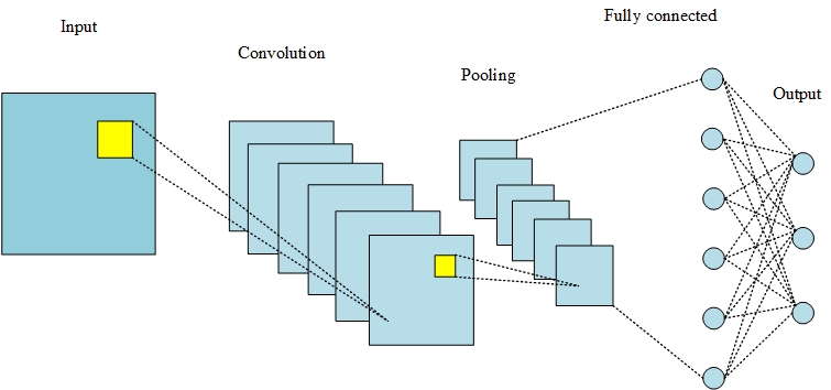
Figure 3. CNN architecture
3.4 Noise Filtering
The OptiKalFilter technique is employed for noise filtering in speech signals. It utilizes an optimized Kalman filtering approach, which is a recursive filter that estimates the true state of a system based on noisy measurements. Advanced optimization techniques are applied to enhance the performance and efficiency of the Kalman filter, resulting in improved noise reduction and speech enhancement.
Kalman Filter
Kalman filtering also appears in neural-network-assisted robot navigation and autonomous-vehicle object tracking, where recursive state estimates serve different measurement models. Its use here concerns noise-corrupted signal processing.
A Kalman filter recursively estimates a system state from a dynamic model and noisy measurements. The prediction stage propagates the previous state estimate and covariance. The update stage combines that prediction with the current observation using the Kalman gain. The supplied formulation is presented below.
Prediction State:
\(\widehat{x_{h}^{-}} = \ \ A_{h}\widehat{x_{h – 1}} + B\ u_{h}\)
\(\widehat{P_{h}^{-}} = \ A_{h}P_{h – 1}A_{h}^{T} + \ Q_{h}\)
Here, Ah is the transition matrix, B is the control-input matrix, uh is the control input, and Qh is the process-noise covariance. The supplied hybrid optimization procedure is used for covariance tuning.
Update state
The measurement update combines the predicted state with the innovation, which is the difference between the observed measurement and its prediction. The Kalman gain determines the contribution of that innovation, and the covariance is updated accordingly.
\(K_{h} = \ \widehat{P_{h}^{-}}U_{h}^{T}{(U_{h}\widehat{P_{h}^{-}}U_{h}^{T} + \ R_{h})}^{- 1}\ \ \)
\(\widehat{x_{h}} = \ \widehat{x_{h}^{-}} + \ K_{h}\ (z_{h} – \ U_{h}x_{h}^{-})\)
\(P_{h} = \left( I – \ K_{h}\ U_{h} \right)\ \widehat{P_{h}^{-}}\ \)
Here, Uh is the observation matrix, Rh is the observation-noise covariance, Kh is the Kalman gain, and I is the identity matrix.
Result and discussion
The supplied implementation uses MATLAB and reports evaluation with UrbanSound8K [11]. The dataset contains 8,732 labeled urban-sound excerpts of up to four seconds across ten classes, including air conditioning, car horns, children playing, dog barking, drilling, engine idling, gunshots, jackhammers, sirens and street music. The manuscript reports a 70% training and 30% testing split. ConvRecGRU is compared with CNN, RNN, GRU, Bi-LSTM and LSTM baselines using accuracy, precision, recall, F-measure, sensitivity, specificity, negative predictive value, false-positive and false-negative rates, and Matthews correlation coefficient. The original reported values are retained below.
4.1 Performance Metrics
The classification measures are defined using true positives (TP), true negatives (TN), false positives (FP) and false negatives (FN). For a multiclass task, these terms must be interpreted relative to a specified positive class or a stated averaging method.
TP counts positive examples correctly predicted as positive.
TN counts negative examples correctly predicted as negative.
FP counts negative examples incorrectly predicted as positive.
FN counts positive examples incorrectly predicted as negative.
The analysis of the performance measures included in the planned and existing analyses is expressed mathematically as follows:
Accuracy
Accuracy is a metric that generally describes how the model performs across all classes. It is useful when all classes are of equal importance. It is calculated as the ratio between the number of correct predictions to the total number of predictions.
\(\ Accuracy = \ \frac{TP + TN}{TP + TN + FP + FN}\) (1)
Specificity
It is known as true negative rate, measures the proportion of negatives which are correctly identified.
\(Specificity = \ \frac{TN}{TN + FP}\) (2)
Sensitivity
It is known as true positive rate, measures the proportion of positives which are correctly identified.
\(Sensitivity = \ \frac{TP}{TP + TN}\) (3)
Precision
The precision is calculated as the ratio between the number of Positive samples correctly classified to the total number of samples classified as Positive (either correctly or incorrectly). The precision measures the model’s accuracy in classifying a sample as positive.
\(Precision = \frac{TP}{TP + FP}\) (4)
Recall
The recall is calculated as the ratio between the number of Positive samples correctly classified as Positive to the total number of Positive samples. The recall measures the model’s ability to detect Positive samples. The higher the recall, the more positive samples detected.
\(Recall = \frac{TP}{TP + FN}\) (5)
F-Measure
It is the harmonic mean of precision and recall
\(F – Measure = \frac{2*precision*recall}{Precision + recall}\) (6)
False Positive Rate (FPR)
A false positive is an outcome in which the model forecasts the positive class inaccurately.
\(FPR = \frac{FP}{FP + TN}\) (7)
False Negative Rate (FNR)
A false negative is an outcome in which the model forecasts the negative class inaccurately.
\(FNR = \frac{FN}{TP + FN}\ \) (8)
Negative Predictive Value (NPV)
Negative predictive value is the proportion of predicted negative examples that are actually negative.
\(NPV = \frac{TN}{TN + FN}\) (9)
Matthews correlation Coefficient (MCC)
Matthews correlation coefficient summarizes the association between the predicted and actual binary labels.
\(MCC = \frac{((TP*TN) – (FP*FN))}{\sqrt{((TP + FP)*(TP + FN)*(TN + FP)*(TN + FN))}}\) (10)
4.2 Performance Analysis
Table 1 compares the supplied ConvRecGRU results with CNN, RNN, GRU, Bi-LSTM and LSTM baselines.
Table 1. Performance comparison of the proposed and existing models
| Sen | Spec | Acc | Precision | Recall | FMeasure | NPV | FPR | FNR | MCC | FRR | TPR | |
|---|---|---|---|---|---|---|---|---|---|---|---|---|
| Proposed | 0.979 | 0.955 | 0.967 | 0.956 | 0.979 | 0.967 | 0.979 | 0.045 | 0.021 | 0.934 | 0.021 | 0.979 |
| CNN | 0.948 | 0.941 | 0.944 | 0.941 | 0.948 | 0.945 | 0.948 | 0.059 | 0.052 | 0.889 | 0.052 | 0.948 |
| RNN | 0.955 | 0.920 | 0.938 | 0.923 | 0.955 | 0.939 | 0.953 | 0.080 | 0.045 | 0.876 | 0.045 | 0.955 |
| GRU | 0.906 | 0.934 | 0.920 | 0.932 | 0.906 | 0.919 | 0.909 | 0.066 | 0.094 | 0.841 | 0.094 | 0.906 |
| Bi-LSTM | 0.899 | 0.885 | 0.892 | 0.887 | 0.899 | 0.893 | 0.898 | 0.115 | 0.101 | 0.785 | 0.101 | 0.899 |
| LSTM | 0.910 | 0.851 | 0.880 | 0.859 | 0.910 | 0.884 | 0.904 | 0.149 | 0.090 | 0.762 | 0.090 | 0.910 |
The table reports sensitivity, specificity, accuracy, precision, recall, F-measure, negative predictive value, false-positive rate, false-negative rate, Matthews correlation coefficient, false-rejection rate and true-positive rate. Sensitivity, recall and true-positive rate describe the same rate under the binary definitions above. The manuscript’s rounded table values and more precise discussion values are retained as supplied.
The proposed model has the highest reported sensitivity (0.9792), specificity (0.9549), accuracy (0.967) and F-measure (0.9674) in this comparison. Its reported false-positive rate is 0.0451, false-negative rate is 0.0208 and Matthews correlation coefficient is 0.9343. The rounded table also places the proposed model above the baselines for precision and negative predictive value. Among the baseline models, CNN has the highest precision (0.941 in the table), while RNN has the highest negative predictive value (0.953). Figures 4–7 illustrate these supplied comparisons.
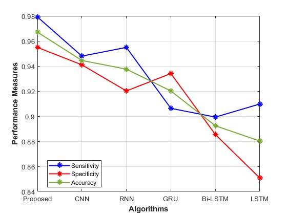
Figure 4. Accuracy, specificity and sensitivity analysis
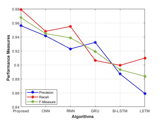
Figure 5. Precision, Recall and F-measure analysis
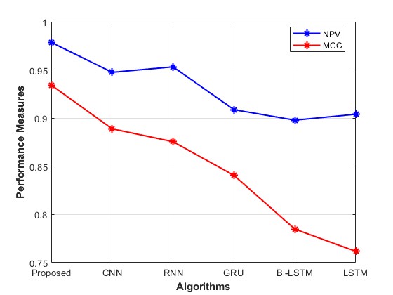
Figure 6. NPV and MCC analysis
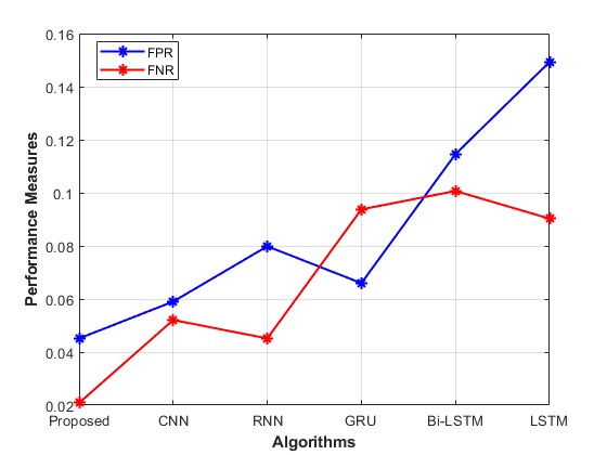
Figure 7. FPR and FNR analysis
Scope and Evaluation Limitations
The supplied results are classification measures. UrbanSound8K is an environmental-sound dataset, and the manuscript does not provide a separate identified clean-speech corpus, an SNR schedule, a fold assignment or perceptual quality scores for its own proposed model. Its reported 70/30 split also differs from the dataset authors’ recommended predefined ten-fold evaluation [11]. The retained scores therefore describe the supplied comparison and do not establish benchmark superiority or independently verify perceptual speech-quality improvement. Further evaluation should specify these details and report intelligibility and signal-quality measures alongside classification performance.
Conclusion
IntelliNoiseFilter combines feature extraction, hybrid neural noise estimation and optimized Kalman filtering. The proposed ConvRecGRU component uses CNN, RNN and GRU representations, while the optimization procedure combines Cat Swarm Optimization with Anarchic Society Optimization. OptiKalFilter supplies the subsequent filtering stage. The supplied results report an accuracy of 0.967 and favorable classification measures relative to the listed baselines. These outcomes support further evaluation of the proposed pipeline within a fully specified and reproducible speech-enhancement protocol.
References
- Shimada, K., Bando, Y., Mimura, M., Itoyama, K., Yoshii, K., and Kawahara, T. (2019). Unsupervised Speech Enhancement Based on Multichannel NMF-Informed Beamforming for Noise-Robust Automatic Speech Recognition. IEEE/ACM Transactions on Audio, Speech, and Language Processing. doi:10.1109/TASLP.2019.2907015.
- Sadeghi, M., Leglaive, S., Alameda-Pineda, X., Girin, L., and Horaud, R. (2020). Audio-visual Speech Enhancement Using Conditional Variational Auto-Encoders. IEEE/ACM Transactions on Audio, Speech, and Language Processing, 28. doi:10.1109/TASLP.2020.3000593.
- Garg, A., and Sahu, O. P. (2020). A hybrid approach for speech enhancement using Bionic wavelet transform and Butterworth filter. International Journal of Computers and Applications, 42(7), 686–696. doi:10.1080/1206212X.2019.1614293.
- Srinivasarao, V., and Ghanekar, U. (2020). Speech enhancement—an enhanced principal component analysis (EPCA) filter approach. Computers & Electrical Engineering, 85, 106657. doi:10.1016/j.compeleceng.2020.106657.
- Yu, H., Zhu, W.-P., Ouyang, Z., and Champagne, B. (2020). A hybrid speech enhancement system with DNN based speech reconstruction and Kalman filtering. Multimedia Tools and Applications, 79, 32643–32663. doi:10.1007/s11042-020-09563-5.
- Dash, T. K., and Solanki, S. S. (2020). Speech Intelligibility Based Enhancement System Using Modified Deep Neural Network and Adaptive Multi-band Spectral Subtraction. Wireless Personal Communications, 111, 1073–1087. doi:10.1007/s11277-019-06902-0.
- Gnanamanickam, J., Natarajan, Y., and Sri Preethaa, K. R. (2021). A Hybrid Speech Enhancement Algorithm for Voice Assistance Application. Sensors, 21(21), 7025. doi:10.3390/s21217025.
- Yu, H., Zhu, W.-P., and Champagne, B. (2020). Speech enhancement using a DNN-augmented colored-noise Kalman filter. Speech Communication, 125, 142–151. doi:10.1016/j.specom.2020.10.007.
- Mahmmod, B. M., Ramli, A. R., Baker, T., Al-Obeidat, F., Abdulhussain, S. H., and Jassim, W. A. (2019). Speech Enhancement Algorithm Based on Super-Gaussian Modeling and Orthogonal Polynomials. IEEE Access, 7, 103485–103504. doi:10.1109/ACCESS.2019.2929864.
- Park, G., Cho, W., Kim, K.-S., and Lee, S. (2020). Speech Enhancement for Hearing Aids with Deep Learning on Environmental Noises. Applied Sciences, 10(17), 6077. doi:10.3390/app10176077.
- Urban Sound Datasets. UrbanSound8K dataset description and evaluation guidance. Official dataset documentation.
Cite This Work
To export a reference to this article please select a referencing stye below:

Academic Master Education Team is a group of academic editors and subject specialists responsible for producing structured, research-backed essays across multiple disciplines. Each article is developed following Academic Master’s Editorial Policy and supported by credible academic references. The team ensures clarity, citation accuracy, and adherence to ethical academic writing standards
Content reviewed under Academic Master Editorial Policy.