Hybrid Deep Learning for Mobility Management in 5G RPL IoT Networks

Abstract

Enhanced Management of Mobility for 5G-Integrated RPL/6LoWPAN IoT Networks leverages a cutting-edge approach involving Hybrid Deep Learning and Savannah Fusion Optimization. The workflow begins with real-time data collection, capturing network metrics, link status, traffic loads, and distances. For Soft Hand-Off, an optimized hybrid deep learning model (combining CNN and DBN) predicts link degradation and network conditions. The CNN weight optimization is achieved through the innovative Savannah Fusion Optimization Algorithm (SFOA), an amalgamation of the African Vultures Optimization Algorithm (AVOA) and Whale Optimization Algorithm (WOA). These algorithms refine hand-off decisions and trigger soft hand-offs when necessary. For Hard Hand-Off, the selection of a backup parent node is optimized using SFOA. Multi-hop add-ons use the optimized hybrid deep learning model to evaluate traffic loads and select optimal routes during hand-offs. Additionally, it integrates loop avoidance and route deferral based on deep learning predictions for efficient and reliable IoT network management.

Keywords: Mobility management; RPL/6LoWPAN; African Vultures Optimization Algorithm; Whale Optimization Algorithm; Soft Hand Off, Hard Hand Off.

INTRODUCTION

Wireless sensor networks constitute a cornerstone of the Internet of Things (IoT) [1], reflecting a substantial stride in AI and a transformative force in modern society [2]. The burgeoning realm of IoT applications, spanning smart cities, transportation, healthcare, environmental monitoring, energy management, and agriculture, underscores the growing demand for seamless mobility support [3]. Traditional Routing Protocol for Lossy Low-power over Low-Power Wireless Personal Area Networks (LoWPANs) inadequately addresses the challenges posed by dynamic topologies [4]. Swift and frequent network topology changes remain unresolved, lacking efficient and precise solutions. A protocol called RPL is based on rank values and relies on an Objective function for determining the path between nodes [5].

The behavior of RPL is affected by different mobility models in distinct ways [6], however, it has been proved that the default RPL protocol degrades quality of service under mobility. IP networks enable seamless end-to-end communication, avoiding the need for gateways and wireless transmission augmentation methods [7]. By utilizing IPv6 addresses, the 6LoWPAN standard does away with the necessity for adaption methods [8][9]. However, multihop 6LoWPAN’s reliability is hampered by instability in wireless communications brought on by things like node failures and constrained capacity [10]. These difficulties affect the overall network performance. The development of RPL/6LoWPAN Networks, with a focus on programmability and scalability to enable QoS provisioning and quick routing configuration in the 6LoWPAN ecosystem, has been sparked by the arrival of 5G.

Location management and handover management are the two main components of mobility management [11]. The latter is concerned with maintaining an IP session for a mobile node continuously while it changes access points [12]. Deep Learning, a kind of machine learning, excels at controlling topologies with a wide variety of network layers [13]. One distinguishing feature of Deep Learning that sets it apart from other machine learning techniques is its capacity to handle networks with an infinite amount of heterogeneous layers. The deep learning model uses only either advanced operations or multiple activations in one neuron. It does not use a simple activation function. The raw input data of the Deep Learning model automatically find the representation and the learning task [14].

There are several methodologies based on IoT-integrated RPL/6LoWPAN Networks for 5G communication. A software-defined networking-based architecture for mobility management has been developed to facilitate swift and precise handovers for nodes in motion within the context of RPL and 6LoWPAN networks. However, a challenge lies in the implementation of precise predictive models, as they demand computational resources beyond the capabilities typically available in mainstream IoT devices [15]. This limitation underscores the need for innovative solutions to strike a balance between predictive accuracy and the resource constraints inherent to IoT devices.

The proposed method is based on the IoT-integrated RPL/6LoWPAN Network for 5G communication by hybrid deep learning-based mobility management. A hybrid deep learning based mobility management method is highly efficient and stronger than the other hybrid methods. The main objectives of the recommended method include,

To improve the speed of the RPL/6LoWPAN Networks.

To analyze the hybrid deep learning-based mobility management.

To integrate the IoT of RPL/6LoWPAN Network for 5G communication by a hybrid deep learning-based mobility management.

LITERATURE REVIEW

Christian Miranda et al., [16], proposed a new intrusion prevention scheme, which effectively prevents Rank attacks in Software Defined Networking (SDN)-based deployment for 6LoWPAN networks using a Reinforcement Learning agent. Thus, their proposed approach achieves cost-efficient route optimization, packet forwarding, and QoS provisioning enhancing packet delivery while ensuring feasible application in software-defined IoT networks remains the core objective.

Ibrahim Alsukayti et al., [17], To prevent and detect version number attacks in RPL-based IoT networks, a collaborative and distributed security strategy have been developed as a simple yet powerful solution. This scheme was built into the protocol design. The solution significantly bolsters protocol resilience against both single and complex VN attacks across diverse experimental configurations. CDRPL offers robust and swift attack detection, coupled with rapid topology adjustment, ensuring the network’s security and stability in the face of any attack endeavor.

Manikannan et al., [18], introduced A mobility-aware, energy-efficient parent selection approach was applied, utilizing the Firefly Optimization Algorithm within the RPL/6LoWPAN IoT network architecture, which yielded remarkable results. The system showcased superior performance in Packet Delivery Ratio, end-to-end delay, and power consumption when compared to alternative systems. Nevertheless, it contains number of hops which is slightly higher when compared to mobility management of RPL+ Particle Swarm Optimization (PSO) and mobility management of RPL+ Ant Colony Optimization (ACO).

Charisma Samuel et al., [19], proposed a novel wormhole detection method for 6LoWPAN networks leverages hop counts and round-trip times. The technique’s performance evaluation encompasses power consumption, CPU utilization, memory utilization, and communication overhead, providing a comprehensive assessment of its efficiency and resource impact within the network. The results display the tunnel created by the wormhole attack has a small impact on both CPU usage and power consumption.

Bacem Mbarek et al., [20], introduced a trust-based detection strategy to combat replication attacks in IoT networks, with a specific emphasis on identifying and mitigating compromised witness nodes alongside testing replica nodes. This approach evaluated the probability of detecting replication attacks and runtime detection performance, comparing Brute-force, Trust-based, and First Visited Strategies. The proposed strategy significantly improved average detection probability to 90% against replication attacks while also mitigating communication failures.

Arya Paul et al., [21], proposed enhanced objective functions developed by various researchers for RPL, a low-power IoT protocol. It systematically assesses the pros and cons of different approaches in objective function design. The study identifies that approaches based on Fuzzy logic exhibit greater efficiency, offering promising advancements in this context.

Sahil Garg et al., [22], proposed a hybrid data processing model which leverages Convolutional Neural Network and Grey Wolf Optimization for efficient network anomaly detection. Thus, the results of an extensive evaluation on benchmark and synthetic datasetsTheir model showcases substantial enhancements with an 8.25% boost in detection rate, a 4.08% reduction in false positives, and a 3.62% improvement in accuracy when compared to conventional GWO and CNN methods.

Aryan Mohammadi Pasikhani et al., [23], proposed an Intrusion Detection System (IDS) for RPL in 6LoWPANs used Reinforcement Learning to identify attacks effectively. This scheme is tailored for resource-limited settings and excels at detecting both novel attacks and mobile intruders, enhancing security in IoT networks with constrained resources. Thus, their proposed method displays the results of experiments comparing the performance of homogeneous and heterogeneous detectors, and also provides security against different internal and external intrusions with low overhead.

Niharika Panda et al., [24], introduced a method called Attack Detection using Support Vector Machine to predict blackhole attacks in WSNs used in the IoT. Their proposed method uses a new dataset for testing the centered on IoT traits. Thus, their proposed method achieves an accuracy of 84.37% in predicting attacks using eightfold cross-validation. Their method is used to identify attacks before they seriously harm the IoT.

Iliar Rabet et al., [25] proposed a lightweight SDN-based mobility management architecture for IoT networks, incorporating an external controller into a constrained IoT network to achieve seamless handoffs during node mobility. Their approach outperformed baseline RPL and state-of-the-art ARMOUR in terms of packet delivery ratio and end-to-end delay, as confirmed through analytical modeling and simulations, with manageable and scalable overhead.

Problem Statement

Although existing literature explores energy-efficient parent selection with consideration for mobility using the firefly optimisation technique in RPL/6LoWPAN IoT networks, a research gap persists in bolstering the number of mobile nodes for real-time 6LoWPAN applications while ensuring network security and various researchers’ advancements in enhancing RPL through improved objective functions there is a research gap in employing machine learning approaches into RPL for optimized computations and enhanced results and establishing methods for dealing with attacks and mobility as well in a Wide Area Network. Attack Detection using Support Vector Machine to predict blackhole attacks in WSNs used in the IoT, there is a research gap in investigating the scalability for larger WSNs. To rectify these research gaps, the proposed method is based on a hybrid deep learning-based mobility management for IoT integrated RPL/6LoWPAN Network for 5G communication. A hybrid deep learning-based mobility management approach is highly efficient and stronger than the other hybrid approaches. By addressing these problems, the research contributes to integrate the IoT of RPL/6LoWPAN Network for 5G communication by a hybrid deep learning-based mobility management, improves the speed of the RPL/6LoWPAN Networks, and analyzing the hybrid deep learning-based mobility management.

System Model

The system comprises two primary phases: (i) the Data Transmission Phase and (ii) the Discovery Phase, depicted in Fig 1. Assuming the Mobile Node (MN) is connected to AP1 with a stable link during the Data Transmission Phase. Periodically, MN assesses link quality by receiving “B” beacons from AP1 and, after accumulating a defined number of data packets, AP1 responds with Average Received Signal Strength or Average Signal-to-Noise Ratio, reflecting radio signal parameters. MN disengages from AP1 under two conditions: (1) deteriorating link quality, based on ARSSI compared to a predefined threshold, and (2) no packet reception, signaled by a time-out mechanism. Subsequently, MN enters the Discovery Phase by broadcasting beacon bursts to neighboring APs (AP2 & AP3) and awaits responses. Upon detecting improved link quality (ARSSI exceeding a threshold), MN switches to the new serving AP (AP2 in this case). The algorithm inherently filters out asymmetric networks by analyzing reply packets in both Data Transmission and Discovery Phases. If an adjacent AP lacks active links, it’s excluded from the process. Smart-HOP optimizes wireless network efficiency through three key parameters: link quality assessment, timeout management, and neighbor AP discovery.

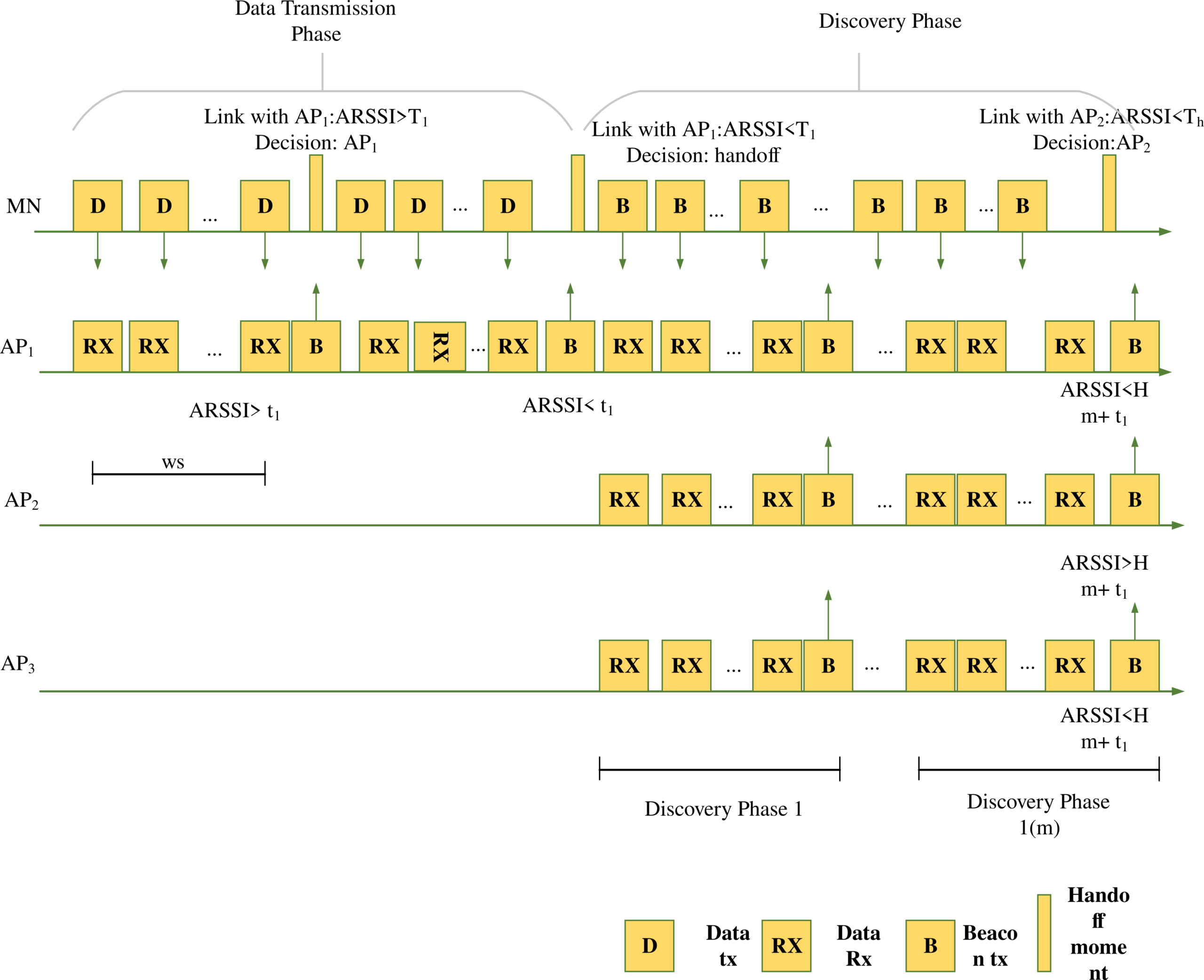
Figure 1 :Smart HOP mechanism timing diagram

Window Size: The Window Size represents the number of packets required for ARSSI computation within a specified time interval.

Hysteresis Margin (HM) : Hysteresis Margin, which establishes t_Land the hand-off initiation ARSSI threshold versus the hand-off termination ARSSI threshold defines the range within which hand-off decisions are made.

t_H≝t_L+HM

Stability Monitoring(m)

Stability monitoring is crucial due to wireless link variability. When the Mobile Node (MN) identifies an Access Point (AP) with ARSSI above Th, it may still drop below Th soon after handover. To prevent this, the candidate AP’s stability is assessed. After detecting such an AP, MN undergoes m additional Discovery Phases to confirm its stability. Notably, the hysteresis margin parameters and stability monitoring are interconnected. A broader HM necessitates a reduced m, and conversely, a narrower HM requires a higher m to ensure effective handover decisions and maintain network stability.

In LPWNs (Low-Power Wireless Networks), selecting appropriate hysteresis margins and thresholds critical and influenced by the transitional region’s characteristics and wireless link variability. This transitional region is often notably extensive, with over 50% of network links being unreliable. Consequently, nodes frequently operate within this transitional region. Empirical experiments have identified the RSSI transitional region boundaries within 92 dBm to 80 dBm is the measurement range.

Setting the threshold (T`) too high can lead to unnecessary handovers, as the node becomes overly selective. Conversely, setting it too low may result in reliance on unreliable links. The hysteresis margin is crucial for managing low-power wireless link variability. A narrow margin (e.g., 1 dBm) can cause frequent, needless handovers (ping-pong effect), while an overly wide margin (e.g., 10 dBm) may lead to prolonged handovers, increasing network inaccessibility periods and reducing delivery rates. Careful parameter selection is thus essential for network performance optimization.

An Overview of DoRPL

RPL, Deep learning, and metaheuristic algorithms are so-called DoRPL, Smart-HOP integration with RPL routing, introduces significant changes to enhance wireless network performance. DoRPL, the fusion of smart-HOP into RPL routing, confronts several key challenges. Parameter tuning is intricate, demanding adjustments to thresholds, margins, and timers to accommodate the nuances of low-power wireless links. Managing transient link quality fluctuations presents complexities, as links that briefly meet quality criteria may degrade post-handover. Control message overhead and network congestion must be carefully managed. Scalability, security, and optimizing the Discovery Phase are persistent concerns. Striking a balance between energy efficiency and frequent link assessments is vital, and adapting to dynamic network conditions remains a challenge, all while ensuring compatibility with diverse LPWN technologies. Figure 1 provides an illustrative example of DoRPL’s timing behavior involving a Mobile Node and three Access Points. During both Data Transmission and Discovery phases, reply beacons from the serving and nearby APs are unicast DIO packets. In the Discovery Phase, bursts of beacons are multicast DIS messages, eliciting DIO responses within specified time windows. This link management process, involving link retention, evaluation, and removal, closely integrates with the Smart-HOP mechanism.

When the Mobile Node detects satisfactory link quality, it remains in the Data Transmission Phase. The Discovery Phase is triggered only upon ARSSI deterioration. Unlike the smart-HOP approach, MN continues data transmission with the serving AP until a superior AP is found. Following a seamless handoff, the RPL algorithm nullifies, ensuring smooth network operation and optimal AP utilization.

During the Discovery Phase, the Mobile Node) initiates a series of DIS control messages, transmitting them to neighboring Access Points (APs) without causing conflicts. Each AP sends a unicast DIO reply containing its ARSSI level. The MN then compares this ARSSI value to a predefined threshold, T_h. If it falls below T_h, When signaling a suboptimal link, the Mobile Node (MN) persists with periodic DIS bursts, synchronized with the Handover Timer. However, when the MN identifies a high-quality link (ARSSI exceeding T_h ), the Discovery Phase concludes, and normal data communication resumes with the newly preferred parent AP in the Data Transmission Phase.

Framework for Mobility Management

To developed a holistic mobility management framework in multi-hop LPWN, emphasizing reliability, efficiency, and timeliness to ensure seamless mobility. This framework encompasses several key components: (i) the design of two handover strategies, both soft and hard handovers, (ii) the development of mechanisms aimed at enhancing handover efficiency, referred to as handover features, (iii) improvements to the RPL routing protocol to optimize end-to-end through the use of multi-hop add-ons, performance during mobility and (iv) a rigorous evaluation of the framework’s outcomes.

Hand-off models

Handover models tailored for the resource-constrained environment of LPWNs, focusing on swift parent switching when link quality degrades. Firstly, use a hybrid deep learning approach, merging Deep Belief Networks and optimized Convolutional Neural Networks to predict link degradation and network conditions accurately. CNN’s weight optimization employs the innovative Savannah Fusion Optimization Algorithm (SFOA), combining African Vultures Optimization (AVOA) and Whale Optimization (WOA) algorithms. To refine handoff decisions, optimization algorithms, particularly SFOA, are applied to select the most suitable backup parent node. A hard handover, facilitated by DoRPL within RPL, acts as a reliable backup if it is necessary. These models are seamlessly integrated into the RPL framework to enhance LPWN performance.

Hand-off features

The design and implementation of algorithms aimed at providing efficient and responsive support for handover models, and achieving backward compatibility by seamlessly accommodating without interfering with the standard RPL methods, mobile nodes can operate within the RPL routing system. In this dynamic environment, ensure rapid handover decisions, facilitated based on the freshness parameter, guaranteeing the use of recent information. Information gathering from neighboring Access Points is carried out without interfering with other activities. To enhance handover efficiency and expedite the detection of parent unreachability and link degradation, four timers within the system. These measures collectively optimize handover operations in LPWNs.

Multi-Hop network

In the context of multi-hop networks, our multi-hop add-ons address several critical considerations within the handover process. During handover, incorporate network metrics, ensuring avoidance of Access Points with heavy traffic loads. Prioritise APs that are closer to the destination simultaneously to enhance route selection. After a handover event, actively prevent loop formation (loop avoidance) and delay route establishment to avoid path breakage (route establishment deferring). These multi-hop enhancements not only improve handover efficiency but also contribute to overall network stability and performance in LPWNs.

Evaluation

Researchers assess the suggested mobility management using in-depth analytical modeling and simulations and contrast different scenarios in different contexts.

Handoff models

Data collection

The main aim of data collecting in this approach is the network metrics necessary for effective LPWN control. These measurements cover a range of topics, such as traffic volume, link deterioration, and distance data. Link degradation data allows us to evaluate the performance and dependability of connections, while traffic load monitoring helps us comprehend network congestion and resource usage. Distance data is crucial for decision-making about route selection and handover, ensuring effective data transmission inside the LPWN. The overall performance and responsiveness of the network are improved by this comprehensive approach to data collection.

Soft Hand off models

To address the resource constraints, present in the world of LPWNs, have developed specialized handover models, emphasizing swift parent switching when link quality declines:

3.3.1 Advanced Hybrid Deep Learning: This approach harnesses the power of a meticulously optimized hybrid deep learning model that synergizes Convolutional Neural Networks with Deep Belief Networks. This fusion empowers the models to make precise forecasts regarding link degradation and the prevailing network conditions, enabling swift and informed handover decisions.

CNN

The Convolutional Neural Network, a prevalent deep learning technique, excels in processing data with grid-like structures. By harnessing automatic and adaptive pattern learning, CNN highlights local relationships within adjacent data structures, progressing from low to high-level features. This capability makes CNN invaluable for various tasks, particularly image and spatial data analysis.

A convolutional neural network (CNN) comprises three essential layers: convolutional layers, pooling layers, and fully connected layers, enabling complex feature learning. The two phases of this architecture are feature detection and classification. During feature detection, features are extracted using convolution, pooling, and ReLU activation. During classification, predictions are made using fully connected and softmax layers. CNNs are skilled at jobs like picture recognition and other pattern-based analyses thanks to this dual-phase technique, which enables them to automatically learn pertinent features and subsequently generate accurate classifications.

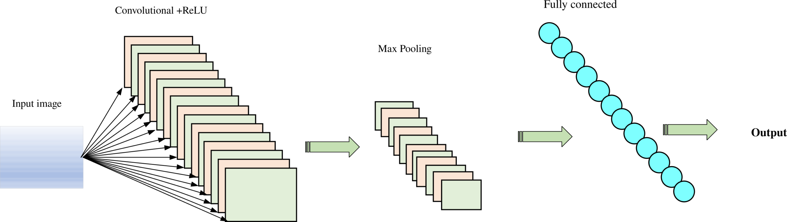
Figure 2: CNN architecture

Convolutional Layer

Within the convolutional layer, the convolution operation involves applying a kernel or filter input tensor to a multidimensional array. The filter, with limited height and width but spanning the input’s depth, serves as a parameterized mask for feature extraction. As the kernel traverses the input tensor’s height and width, it computes scalar products between itself and the covered input portions, generating output values for each position. The culmination of this process creates the activation map, also known as the functionality map, a volumetric representation highlighting learned features through convolutional analysis.

ReLu

A critical non-linear activation function that follows the convolutional layer transfers only activated features to the layer following that. The rectified linear unit threshold elements by performing an operation and keeps positives while converting negatives to zero, is prominently preferred. The effectiveness of this option is demonstrated by its quick learning curve and superior performance to more conventional units like the hyperbolic tangent. ReLU has gained popularity because of its demonstrated prowess in accelerating gradient flow, addressing vanishing gradient issues, and improving deep learning model convergence and general efficacy.

Pooling Layer

In the pooling layer, a non-linear sub-sampling process reduces the spatial dimensions of activation maps while preserving their depth information. Its objectives encompass streamlining the preceding convolutional layer’s output and introducing translational invariance against minor shifts and distortions. This augmentation enhances the feature localization’s robustness. Drawing an analogy to the visual cortex, pooling units simulate complex cell behavior by assimilating expanding visual fields, thereby acquiring spatial hierarchies of feature patterns. Max pooling is a prevalent technique, involving non-linear sub-sampling through partitioning inputs into rectangles and returning maximum values within these windows. Despite its minimal weights, essential hyper-parameters like filter size, stride, and padding shape this layer’s behavior during training. Equating filter size and stride leads to a reduction in the input tensor’s size by a factor of “r.”

Fully Connected layer

Following the final feature extraction stage, activation maps are converted to vectors, then connecting them to one or more completely connected layers. Within these layers, each input vector value connects to all subsequent layer values. The ultimate fully connected layer generates a vector of size K, mirroring the class count for classification purposes. This process streamlines feature aggregation and pattern recognition, enabling the network to make informed decisions and classify inputs into distinct classes based on learned representations.

Softmax Layer

It’s common for the activation function in the final fully connected layer to differ from those in preceding layers, chosen based on the network’s intended task. In multi-class learning, the softmax function normalizes the K actual values obtained from the last FC layer, representing the probabilities of belonging to each of the K classes.

Deep Belief Network

Deep Belief Networks (DBN) stand as unsupervised probabilistic deep learning algorithms, distinguished by their multi-layered structure comprising latent variables that are random. These binary latent variables, commonly referred to as hidden units or feature detectors, serve as the building blocks of the DBN. This generative hybrid graphical model exhibits a unique architecture: The associative memory is formed by connections that are made randomly by the top two layers.

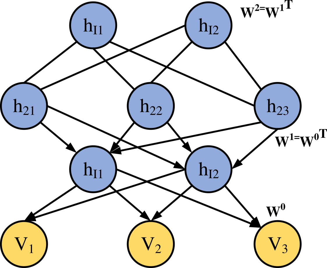
Figure 3: DBN architecture

In contrast, lower layers establish directed connections, with arrows pointing towards the layers closest to the input data. These lower layers form a directed acyclic structure, converting associative memory into observed variables, with the lowest layer receiving binary or real input data. Importantly, unlike Restricted Boltzmann Machines (RBMs), there are no connections between the layers. within a DBN. The hidden units in DBN represent features capturing correlations within the data, while connections between two layers are mediated by a matrix of symmetrical weights, connecting each unit in one layer to every unit in the neighboring layer.

Tailored CNN Weighting: To further enhance model effectiveness, a unique hybrid optimization paradigm, the Savannah Fusion Optimization Algorithm (SFOA). SFOA represents a strategic amalgamation of two robust optimization algorithms: the African Vultures Optimization Algorithm (AVOA) and the Whale Optimization Algorithm (WOA). It serves as a means to finely optimize the weighting of CNN, ensuring that our handover models are not only adept at swift decision-making but also capable of delivering optimal performance within the resource-constrained LPWN landscape.

Hybrid Optimization Model

The proposed hybrid optimization model Savanah Fusion optimization Algorithm (SFOA) is the combination of Standard African Vulture Optimization and the Whale Optimization Algorithm (WOA).

Standard African Vulture Optimization algorithm

The AVOA meta-heuristic algorithm draws inspiration from the feeding and orienting behaviors exhibited by African vultures. These remarkable birds are categorized into two distinct groups, shaped by their physical prowess and natural tendencies. Vultures’ relentless quest for sustenance drives them to spend extensive hours scavenging for food, enabling them to evade the perilous grasp of hunger. Furthermore, the algorithm regards the most formidable and proficient vultures as the embodiment of optimal solutions, embodying strength and superiority in their pursuit.

Deciding which vulture is best for each group

Depending on the fitness function, the first and second vultures are selected for the overall optimisation in the first stage of the AVOA algorithm. The following formula then provides further solutions that indicate the option of choosing the vultures.

r(I)={BestVulture₁ if P_I=∝ ; BestVulture₂ if P_I=β (1)

Before the search operation, the parameters ∝and β in Eq. (1) and are quantized. These parameters encompass a scale from 0 to 1, and when summed, they collectively hold a significance equivalent to 1. The selection process employs a roulette wheel mechanism to choose from among the most optimal choices available. As the value of ∝ approaches unity, the degree of exploitation experiences a substantial increase. Eq (2) precisely defines the vulture’s vitality rate, factoring in its behavior, energy deficiency, and aggressiveness during the pursuit of sustenance.

f=(2×rand₁+1)×Y×(1-(IT_I)/(maxIT)) (2)

f in Eq. (2) represents the vulture’s level of satiety. IT_I represents the maximum iteration number at this time. It is the overall number of repetitions, while y is a random value between 1 and 1 that varies with each iteration. The vulture is hungry when Y is less than 0, else there aren’t any vultures; rand1 is a random number between 0 and 1. Exploration and exploitation are balanced by the value of the variable f in the AVOA algorithm.. The exploration phase begins when the value of |f| exceed 1; otherwise, the exploitation phase begins.

Phase of Exploration

During this stage of the AVOA algorithm, population exploration and diversity are crucially influenced. Depending on the value of the parameter P1, ranging from 0 to 1, two strategies are adjusted. When the random number P1 (generated between 0 and 1) is greater than or equal to a specified parameter, Eq. (3) is employed, and Eq. (4) is used when P1 is smaller, to choose any of the exploration phase strategies.

v(I+1)=r(I)-d(I)×f

(3)

d(I)=|x×r(I)-v(I)|

Eq. (3) suggests that v(I+1) is the vulture’s position vector evolves. f represents the vulture’s satiety level, while r(I) designates the top-selected vulture. The variable xdenotes the leader vulture’s unpredictable movement to protect food from others, calculated as x= 2rand where rand is a random value between 0 and 1. This x serves as a coefficient vector, augmenting random motion that varies with each iteration. vI corresponds to the current location vector of the vulture, collectively contributing to the dynamic behavior of the vultures during the optimization process.

v(I+1)=r(I)-f+rand₂×((ub-lb)×rand₃+lb) (4)

between 0 and 1 at random is rand₃ in Eq. (4). The lower and upper boundaries are also represented as lb and ub. In order to increase the random quiddity coefficient, rand₃.

Exploitation Phase

At this point, the AVOA algorithm defines convergence and efficiency. The two parameters p2 and p3 are taken into consideration as two methods with values between 0 and 1 are modified at this stage. In the next section, each exploitation phase approach is listed.

Phase 1

The initial phase employs two additional tactics: rotation flight and silent quarrel, each offering distinct strategic advantages.The p2 parameter is represented as Eq (5)  to determine which method is chosen. that randp2 is an arbitrary number between 0 and 1.

v(I+1)={Equation(6)if p₃≥rand_P2 ; Equation(8)if p₃<rand_P2 (5)

A quiet quarrel and Siege

The severe disagreements over food acquisition between weak and important vultures begin at this point in the AVOA algorithm, as shown by Eq. (6).

v(I+1)=d(I)×(f+rand₄)-D(T) (6)

D(T)=r(I)-v(I) (7)

Eq. (6) increases the random coefficient by rand₄, a random number between 0 and 1. , r(I)was one of the two groups of vultures that was picked with the most care. The vulture’s present vector location is v(I). This equation can be used to calculate the separation between the vulture and one of the top vultures in the two groups.

The vultures’ rotational motion

In this stage of the AVOA algorithm, rotational motion is emulated through spiral movement. The algorithm calculates the distance between a vulture and one of the top two vultures. Additionally, it constructs a spiral equation guiding the vulture’s movement towards one of the largest vultures, adhering to the principles of natural flight f dynamics.

v(I+1)=d(I)×e^sf×cos((2πf))+r(I) (8)

s is a parameter applied in Eq. (8) to determine the spiral’s logarithmic model.

Phase 2

The direction of the food source towards which all vultures are moving is monitored in this stage of the AVOA algorithm. Eq. (9), in which rand_P3is a random number between 0 & 1 is the formulation for the P2 parameter, which is used in determining the selection rate of each of the methods.

v(I+1)={Eq11 if p₃≥rand_P3 ; Eq12 if p₃≥rand_P3 (9)

Numerous vulture species are circling their food source.

At this stage, every vulture’s movement towards the source of food is being observed. Equations (11) and (12) are used to represent the behaviour of hungry vultures, which engage in severe competition for food and may congregate around a single food source.

a₁=BestVulture₁(I)=d(I)×f

(10)

a₂=BestVulture₂(I)=d(I)×f

BestVulture₁(I), in Equation (10), refers to the dominant vulture in the first group at this time, and BestVulture₂(I), to the dominant vulture in the second group at the moment.

v(I+1)=(a₁+a₂)/(2) (11)

Equation (11) is applied to aggregate all vultures.

Fierce and Siege quarrels

In this phase of the AVOA algorithm, the dominant vultures exhibit signs of frailty and hunger, emphasizing their pivotal role , but they are also engaged in heated disputes. also approach the leading vulture from different angles. Modeling of this movement has been done using Equation (12).

v(I+1)=r(I)-|D(T)|×f×Levy(D) (12)

The distinction between the top vultures in each group and the vulture is indicated by the variable D(T) in Equation (12). The flying patterns of the levy flight function have been used to improve the performance of the AVOA algorithm in Eq. (12).

Whale optimization Algorithm

Whale Optimization Algorithm is a population-based optimization technique inspired by the social behavior of whales. It uses a multi-objective function to find the global optimum solution.

Three phases make up the WOA algorithm, which formulates the spiral bubble hunting technique used by whales: (1) encircling prey; (2) exploitation and (3) exploration.

Phase of encircling prey: The whales find the prey during this phase, after which they encircle them. From a set of search agents that were generated at random, WOA then chooses the best candidate search agents. In addition, other whales make an effort to change their positions in light of the currently listed best candidate. In order to formulate the entire procedure, the following Eqs. (1) and (2) are used:

C⃗=|D ∙⃗ A⃗ (s)- A⃗(s)| (13)

A⃗(s+1)= A ⃗(s)- X⃗ ⋅C⃗ (14)

where t stores the current iteration, X⃗ and D⃗ stand in for coefficient vectors, the A^*⃗vector denotes the correct solution position vector discovered up to this point, and A ⃗denotes the position vector. Using Eqns. (15) and (16), The X⃗ and D⃗ coefficient vector values will be calculated.

X ⃗=2x⃗⋅f ⃗-x⃗ (15)

D⃗=2. f ⃗ (16)

where, over the course of the algorithm iterations, the variable x⃗ value decreases linearly from 2 to 0.. Additionally, the vector f ⃗denotes a random value between 0 and 1.

Phase 2: Exploitation: This phase is based on two techniques: spiral updating position and shrinking encircling technique.

Technique of shrinking the circle: They develop the shrinking encircling behaviour by reducing! a variable that ranges linearly from 2 to 0 and is used in Eq. (15) over the course of the algorithm iterations, corresponding to the value ofX ⃗ A random value over [-x, x] is a vector.

Position updating spiral : They determined the whale’s behavior by measuring the distance between the whale and its prey. Using Equation (17), they modeled the whale’s spiral motion as it moved from its current spot to the prey’s location based on this distance calculation.

A⃗(s+1)= C⃗⋅e^yj⋅cos((2πj))+ A^* ⃗(s) (17)

where A ⃗= |A^*⃗ (s)-A⃗(s) |,this distance represents the gap between the present whale position and its prey. When studying humpback whale behavior around prey, it was found that these whales employ both shrinking circling and spiral movement techniques simultaneously. Furthermore, an equation is employed to gauge the likelihood of whales switching between these two behaviors, with a 50% probability.

A⃗ (s+1)= {A^* ⃗(s)-X ⃗∙ C⃗ if q<0.5 ; C⃗⋅e^yj⋅cos((2πj))+ A^* ⃗(s) if q≥0.5 (18)

where q is a number drawn at random from [0, 1],

Phase three is exploration (hunting for prey), during which humpback whales conduct a worldwide search in exploration.

The X ⃗ value determines whether the phase is an exploration or an exploitation; if the X ⃗ is larger than or equal to 1, the phase is an exploration. If not, the phase is an exploitation. Instead of updating their position to the best whale for a global search during the exploration phase, the whales update it in relation to a randomly chosen whale. Eqs (19) and (20) will therefore be used to calculate the whale’s new position.

C ⃗= |D ⃗∙A_rand⃗- A⃗| (19)

A⃗(s+1)=A_rand⃗- A⃗ ∙C⃗ (20)

X_rand represents a randomly selected whale’s location from the available group of whales.

Multi Hop AddIns with hybrid deep learning

Optimal Route Selection

In this network architecture, the selection of the optimal route is pivotal for network efficiency. When the mobile node (MN) packets must be forwarded to the root, it intelligently picks the Access Point with the lowest rank. This choice minimizes the number of hops data packets must traverse to reach the root, thereby reducing end-to-end delay. However, for transmitting data to router/leaf nodes, MN Needs data on accessible routes to nearby Access Points (APs). Traditionally, RPL routing directs packets towards a single router (the root) within a Directed Acyclic Graph (DAG). Nevertheless, design accommodates the establishment of direct communication between any two routers, even if neither of them serves as the root node. This communication mode, termed point-to-point (P2P), functions via a responsive mechanism akin to AODV routing. Messages are appended to DIO packets and distributed using the Trickle algorithm, establishing a transient DODAG (Destination-Oriented DAG) oriented towards the target. Interestingly, whether selecting the root node or any router as the destination, handover performance remains unaffected, albeit potentially influencing overall network efficiency. This is due to all routers possessing routing path information to the destination, enabling the mobile node to make informed neighbor AP selections.

Moreover, each access point (AP) incorporates mobile destination addresses within DIO messages seamlessly, without introducing extra communication or computational burdens. In the context of RPL routing, this integration operates smoothly. When neighboring APs send DIOs, the mobile node (MN) identifies the AP that possesses a route to the intended destination. Confirmation of a viable path from an AP to the specified destination relies on the presence of the destination address within the received DIO message. In cases where the selected AP lacks a direct path, packets are routed through the root and then channeled down to reach the target destination, ensuring efficient communication within our network framework.

After a handoff, multi-hop add-ons

During a hand-off operation in RPL, parent switching can disrupt the routing tree. To maintain prevent loops and descending routes after mobility, two methods are introduced: route establishment deferral and loop avoidance. These techniques help ensure smooth and efficient routing adaptation in response to mobile node movement within the network.

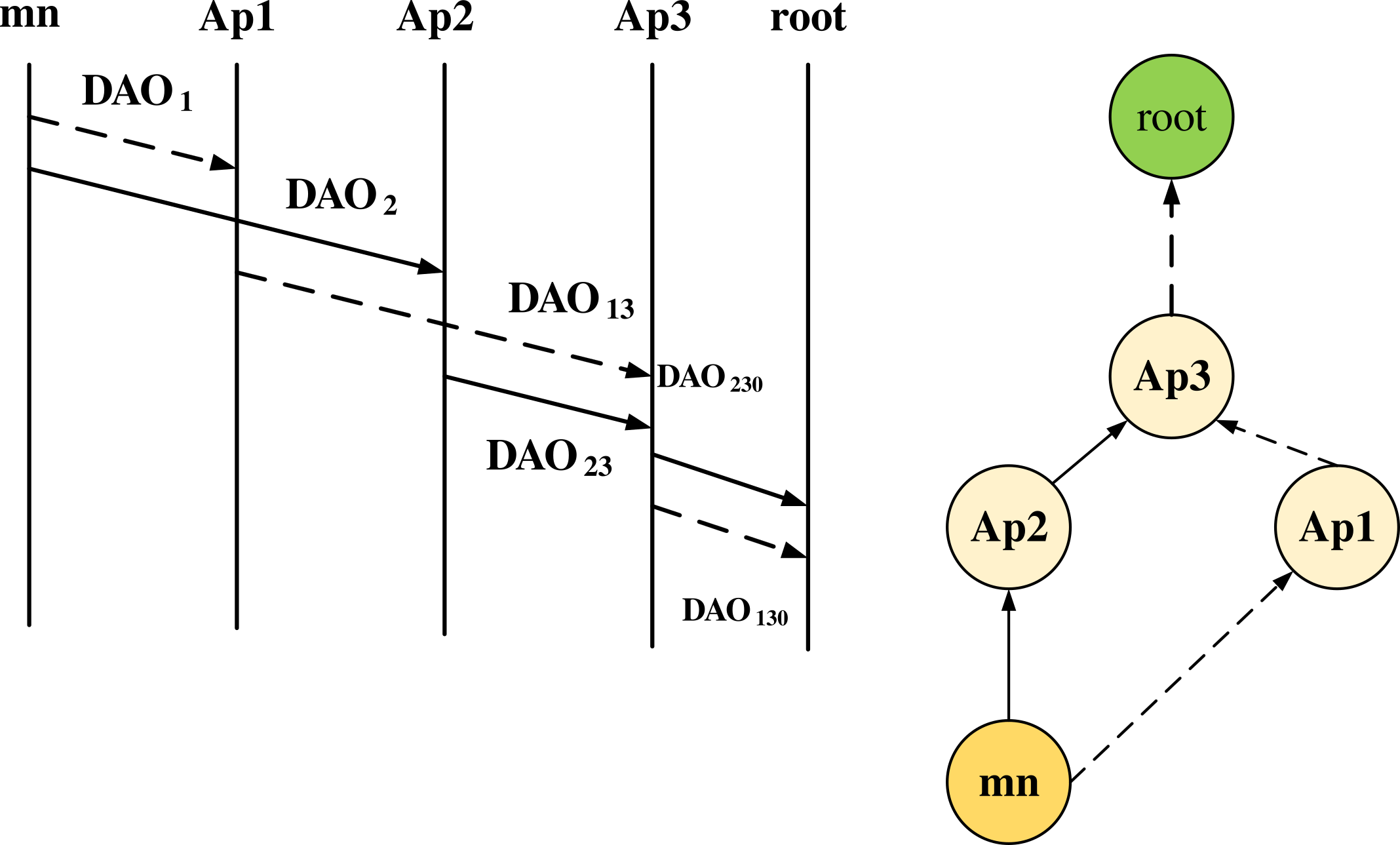
Figure : 4(a) Default Mechanisms for DAO Transmission in RPL

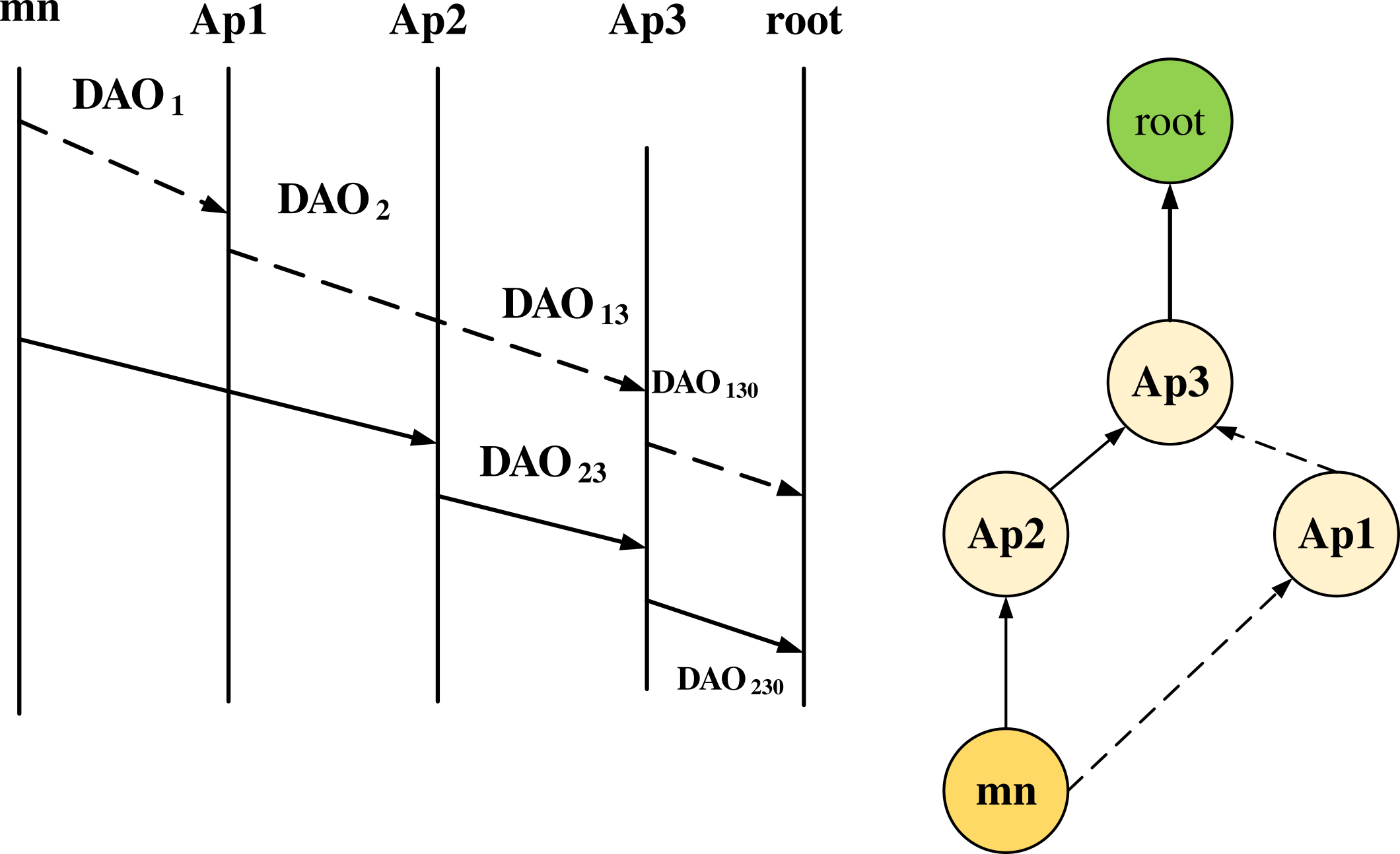
Figure :4 (b) Strategies for Path Preservation Through DAO Deferral in RPL

Route establishment deferring

Lower routes may not work after a hand-off procedure. Data connection from the destination towards the MN will be affected downward due to this issue. There are numerous situations where two-way communication is advantageous. In clinical monitoring, for instance, if the source and destination nodes are both mobile nodes (patients and nurses/doctors), the destination may ask the source node for a measurement.

Following a handover in which an MN transitions from one parent to another, the process of forging new descending routes begins with the unicast of DAO control messages. To sever the previous downward route, the MN initiates a DAO message directed to the former AP, advancing towards the target node to dismantle the entire path. Subsequently, the MN sends a second DAO message to the new AP to establish a fresh route.

An MN going from the area of AP1 towards AP2 in Figure 4(a) is an illustration of a route being constructed in RPL after a parent switching. A DAO message is unicatted to AP1 by the RPL routing, followed immediately by another DAO message for AP2. Up until it gets there, the DAO signal is routed by intermediate APs. In some circumstances, a lengthier processing or communication latency would cause the DAO transfer to be delayed. As a result, a shared link between AP1 and Before moving the AP2 may initially employ the DAO to disconnect the existing downward link before redirecting it towards the construction of a new downward link. All packets sent from root to the source node are discarded as a result of the route breakage caused by this problem. Therefore postpone the DAO transmission for (t period) after constructing a new downhill path in accordance with Algorithm 1 to lessen the likelihood of downward link breaking. In order to maximise the likelihood of the downward connection establishing towards the new serving parent, Figure 4(b) illustrates the scenario where the DAO transmission to AP2 is postponed.

Loop avoidance

In RPL, when a node detaches from its parent, its rank value is altered to an infinite value (e.g., from 20 to ∞). Consequently, the mobile node (MN) can potentially connect with lower-ranked nearby nodes. If the routing table is globally updated across all routers, as in default RPL, this approach effectively eradicates routing loops.

A local routing table update could result in routing loops, though, as the global routing table update is very time- and energy-intensive. For instance, the MN might decide to choose a neighbour node as the new parent even though that node was once the MN’s kid . The MN is free to select the neighbour because it has a lower rank than the infinity, which is determined by the default RPL.

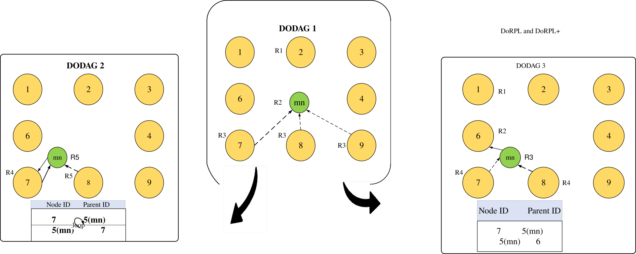
Figure 5: Diverse DODAG Update Strategies: Mobility, Standard RPL, and DoRPL

According to Figure 5, Node 5 in DODAG 1 has three offspring, Nodes 7, 8, and 9, as well as a parent, Node 2. A node of lower rank (shown next to each node) receives input from each node. In the context of RPL routing, DODAG 2 forms when Node 5 leaves from Node 2’s communication range. During this event, the mobile node (MN) selects a neighbor with the highest ARSSI level while setting its rank to infinity initially. Consequently, Node 7, formerly a child of Node 5, becomes the preferred parent with a rank level of 6. However, this choice inadvertently creates a closed loop when data messages from Node 5 are redirected to Node 7, potentially causing routing inconsistencies, which then forwarded the messages back to Node 5 (its parent).

In this context, we’ve developed an effective loop avoidance mechanism outlined in Algorithms 2. Evaluated two distinct approaches to prevent loop effects during handovers. The Mobile Node (MN) adopts a two-step approach for parent selection in DoRPL+. Initially, it receives responses from neighboring Access Points (APs) and excludes messages from its former children when considering alternative parents. Secondly, the children abstain from responding to join requests from their previous parent. This minimizes communication overhead during handovers. When the Mobile Node (MN) disconnects from its current Access Point (AP), its rank resets to infinity. Subsequently, it receives high-quality probes from neighboring APs and joins the AP with rank R, subsequently updating its rank to R + 1. This loop avoidance mechanism is illustrated in DODAG 3, where Node 5 transitions from Node 2 to Node 6, bypassing its previous children. This enhancement is integrated into both mRPL and DoRPL+ models.

“Additional hand-off features”

To create an efficient, low-overhead hand-off architecture, two critical features were developed. First, backward compatibility allows easy integration of hand-off processes into RPL routing. Second, collision avoidance minimizes the risk of control message clashes during hand-offs, guaranteeing smoother and more dependable transitions in wireless networks.

Backward compatibility

To ensure smooth coexistence between mobility-enabled RPL nodes and default RPL nodes without interrupting Trickle timers, enhancements are made to existing RPL control messages. Additional bits in DIS and DIO messages serve two key purposes: distinguishing hand-off control messages from regular ones and conveying essential information such as link quality and a list of destinations with paths to the Access Point for optimal route selection.

A one bit flag is implemented to differentiate between the DoRPL DIS and the standard RPL DIS packet – see Figure 6(a). The RPL DIS multicast transmission is represented by initialising this field to “0”. To reflect the unicast DoRPL DIS broadcast, set this field to “1”. The extra two bits of “C” refer to the window size’s DIS message counter. The counter, for instance, advances to a maximum of 3 when ws = 3.

Two new fields are added to the DoRPL+ DIO messageTwo crucial fields in the message are: (1) F-DIO,two key fields in the message are: (1) F-DIO, representing flags, and (2) ARSSI, containing the average RSSI reading from the potential parent node, as depicted in Figure 6(b)

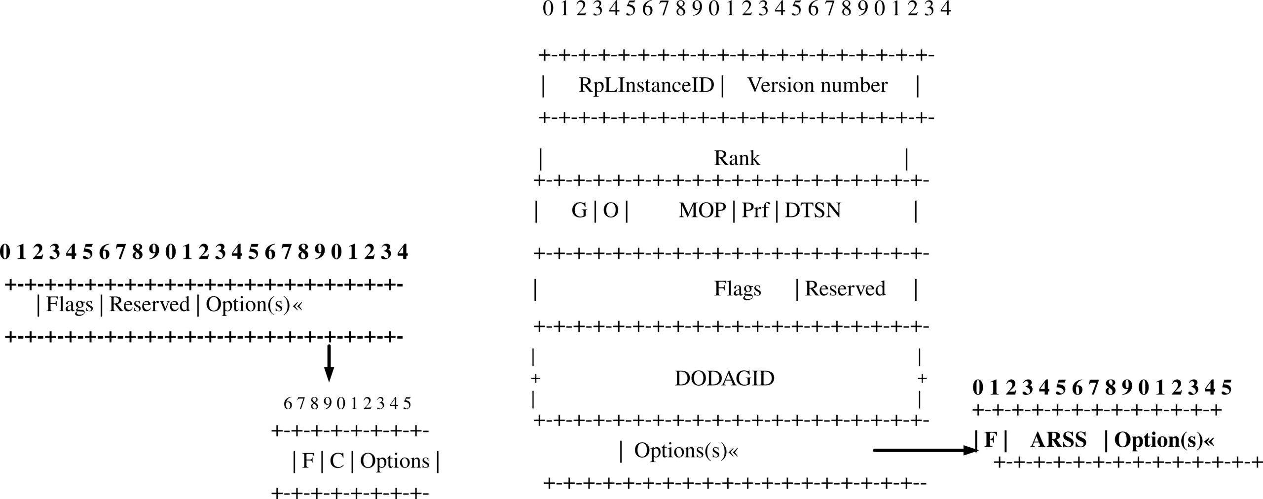
Figure 6 :Enhanced DIS and DIO Packet Formats with F-DIS, C, and ARSSI Fields for Improved RPL Operation

Three cases are distinguished by F-DIO’s two bits: The RPL DIO is represented by (i) F-DIO=0 denotes DoRPL DIO during the Data Transmission Phase. (ii) F-DIO=1 signifies DoRPL DIO in the Discovery Phase. (iii) F-DIO=2 corresponds to a distinct DoRPL DIO condition.

Collision avoidance

In order to exchange packets with the adjacent APs, the MN, this procedure offers a conflict-free medium, use two key techniques to lessen the probability of collision: Poor linkages (ARSSI Th) choose not to inform the high-quality Aps and MN, respond earlier than low-quality APs during designated time periods. The collision avoidance system is described in Algorithm 3. To distinguish between the link settings for high and low priority links, add a new parameter called “prio”. Only 0 and 1 are valid inputs for prio. For measurements of higher quality (ARSSI% “85 dBm), it sets to 0, and for measurements of lesser quality (“85 dBm ARSSI “80 dBm), it sets to 1. It is possible to measure high-quality links at many neighbour APs, which would cause those APs to set prio = 0. To choose various time slots for transmitting DIO packets, take into account an additional random delay (rand(t1, t2)). The limits of the random delay are t1 = 10 ms and t2 = 15 ms, which are longer than the maximum time that IP-based packets can be transmitted (4 ms) using IEEE 802.15.4 radios.

This formula determines the delay in transmitting DIO responses: T_offset = T₂ ×prio + rand(T₁,T₂). In the worst case situation, a poor link (prio = 0) delays sending a DIO packet to the MN forT₂ ⌈(prio ×T₂+rand(T₁,T₂))⌉=T₂ before doing so.

In order to avoid extremely high or extremely low AP densities, researchers are exploring a sensible AP deployment in our system model. Our tests ensure that there is a minimum amount of overlap between adjacent APs, hence eliminating the potential of having many high-quality APs in a given area. DIO packets cannot be transmitted concurrently with other packets using the suggested collision prevention approach.

Freshness. It’s critical to base hand-off decisions on factual information. The hand-off is initiated in a mobile network based on link quality data. Mobile node movement causes a dynamic change in the links in low-power networks. As a result, record the time-stamp of each message sent by a different AP along with its address and ARSSI metrics. The information from this AP is deleted from the buffer when a time window (such as 500 ms) has passed. With this straightforward method, environmental dynamics have less of an impact on the link quality data.

TimersAll nodes establish timers for various purposes: (i) to identify current AP link degradation by prompting replies, (ii) to detect parent unreachability by requesting responses during idle link periods, (iii) for handling neighbor AP replies in soft and hard handoff scenarios, and (iv) to regulate request periodicity in bursts during the swarm’s discovery phase.The following is a quick description of these times.

Connectivity timer (t_c) Mobile nodes use this timer to continuously check whether an AP is providing clients. The MN continues to monitor packets arriving from the serving parent during this time while continuing to listen to the channel. If the MN notices a silent parent after the TC has expired, it initiates the Discovery Phase. Resetting the serving AP connectivity timer after detecting any packet reception.

Mobility detection timer (t_md) Packet loss can be caused by node movement and disconnection owing to the presence of outside objects. In the quest for a new serving parent, the Mobile Node triggers the Discovery Phase. The mobility detection timer’s frequency hinges on the data generation rate, efficiently facilitating handoff and parent selection, dynamically adapting to the ever-changing mobility patterns encountered by the Mobile Node.

Timer for Handoff (t_ho) This timer controls the frequency of sending DIS bursts to the nearby parents. During this time, it is possible to send DIS bursts at their maximum rate and receive sporadic responses from nearby nodes. Each burst’s DIO responses are immediately gathered after being sent. Each parent’s response sequence is planned in such a way as to lessen the likelihood of a collision.

Timing response ( t_r)

During specific intervals, the serving parent must unicast a DIO control message to respond to the Mobile Node (MN). Timing is critical, as an incorrect response time may lead to collisions with data packets, initiating the discovery phase. The parent node gathers essential data, such as the packet count within various window sizes. The reply time computation employs the formula (WS-c)×t_dis, where C denotes the DIS packets within each window size (WS), and t_dis, represents the DIS interval. This reply time adapts dynamically with the reception of each new packet, ensuring efficient communication.

The parent node collects relevant data, like the number of packets in each window size. The reply time is calculated using the formula(WS-c)×t_dis, where C represents the DIS packets within each window size (WS), and t_dis, signifies the DIS interval. This reply time dynamically adapts with the reception of each new packet, ensuring efficient communication.

Result and Discussion

Experimental Setup

In this research , the proposed model has been implemented in MATLAB and the corresponding outcomes generated have been noted. The handoff delay with different data transmission periods is shown in the table 1.

Table 1 compares the performance of RPL, DoRPL, and DoRPL+ routing protocols while presenting handoff latency measures for various data transmission durations. When the transmission times, which range from 0.05 to 0.1 seconds.,the initial handoff delays of 15 and 16 in the case of RPL(12-8), which thereafter stabilise at 14 for times varying from 0.5 to 1 seconds. However, a sharp increase to 35 and 33 at 2 and 5 seconds suggests possible network inefficiencies or congestion. On the other hand, RPL(8-1) has reduced initial handoff delays of 8 and 8, which increase progressively to 12 and 14, respectively, indicating an easier transition. As a result, handoff delays are roughly constant between 25 and 24, demonstrating the protocol’s reliability and depending on the length of the data transmission intervals.

Table 1: Analyzing Handoff Delay Variations Across RPL Networks with Differing Data Transmission Period

Table 2 shows the handoff delay findings from comparing DoRPL and DoRPL+ routing protocols over a range of data transmission times. Both DoRPL and DoRPL+ display nearly low handoff delays at 0.005 seconds for a data transmission period of 0.05, 0.1, and 0.5. Observe performance variations as the data transfer time increases to 1, 2, and 5. With readings of 0.082, 0.085, and 0.08 seconds, respectively, DoRPL+ retains its minimal delay. DoRPL, on the other hand, shows marginally longer delays of 0.084, 0.083, and 0.079 seconds. These results illustrate DoRPL+’s potential improvements over DoRPL for circumstances involving longer data transfer times.

Table 2: Comparing Handoff Delay in DoRPL and DoRPL+ with Varied Data Transmission Periods

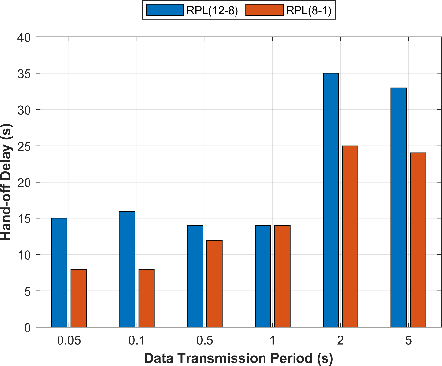
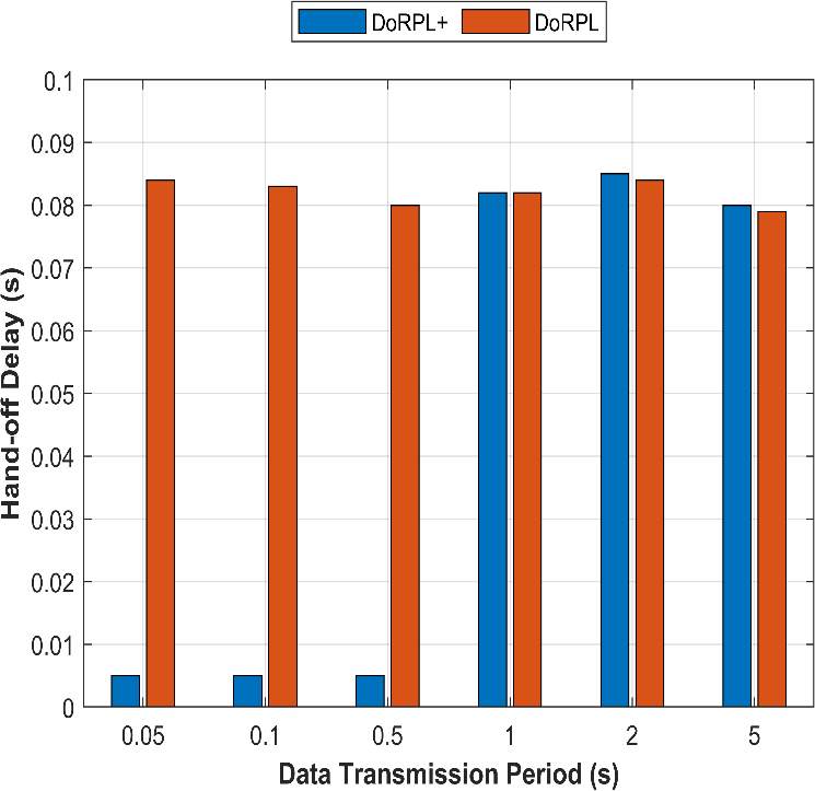
Figure 7: Analyzing Handoff Delay Variations with Diverse Data Transmission Periods: (a) A Comparison with RPL, and (b) Evaluating DoRPL Versus DoRPL+

Table 3 illustrates the total network overhead information for various data transmission times while comparing RPL, demonstrating the effectiveness of two RPL variants: RPL(12-8) and RPL(8-1). RPL(12-8) experiences network overheads of 500, 550, and 555 for data transmission periods of 0.05, 0.1, and 0.5, respectively. RPL(8-1) has greater overheads for the same durations at 5500, 5700, and 5500. Both variants exhibit variances when transmission times increase to 1, 2, and 5, with RPL(12-8) varying from 560 to 545 and RPL(8-1) having a more consistent overhead of approximately 5400. These results illustrate how the two RPL protocols differ in terms of network overhead under various data transfer conditions.

Table 3: Evaluating Network Overhead Variations with Varied Data Transmission Periods in RPL Networks

In table 4 represents the overall network overhead information for various data transmission times with a comparison of the two routing techniques, DoRPL and DoRPL+. DoRPL+ has lower network overhead during data transmission periods of 0.05, 0.1, and 0.5, with values of 590, 612, and 553, respectively, while DoRPL has slightly higher overheads of 620, 620, and 580 for the same intervals. DoRPL+ continuously maintains a lower overhead than DoRPL as by increase the data transmission intervals to 1, 2, and 5, illustrating its potential efficiency advantage in cases with longer data transmission intervals.

Table 4: Assessing Network Overhead Variation Across Diverse Data Transmission Periods period while comparing DoRPL with DoRPL+

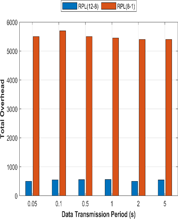
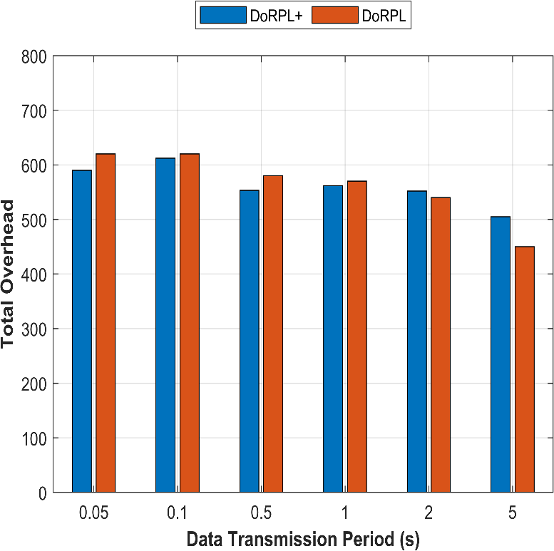
Figure 8: Analyzing Network Overhead with Varied Data Transmission Periods: (a) A Comparative Study with RPL, and (b) A Comparative Assessment of DoRPL and DoRPL+

Different tendencies showed up in this research of RPL’s performance under different data transmission times is illustrated in table 5. RPL(12-8) had a packet delivery ratio of 56% at 0.05 seconds of data transmission, while RPL(8-1) exceeded it with 79%. While RPL(8-1) grew to 81% when the transmission time increased to 0.1 seconds, RPL(12-8) showed a modest decline to 54%. Notably, RPL(12-8) significantly outperformed RPL(8-1) with a transmission period of 0.5 seconds, reaching a delivery ratio of 70%, whereas RPL(8-1) deteriorated to 68%. This pattern continued, and RPL(12-8) continued to be the best, hitting 80% at 2 seconds and 82% at 5 seconds. RPL(8-1) saw a dip, nevertheless, dropping from 69% at 1 second to 60% at 5 seconds. These results illustrate the complex interaction between data transmission intervals and RPL protocols, emphasizing the strength of RPL(12-8) in maintaining packet delivery ratios throughout a wide range of transmission intervals.

Table 5: Comparative Analysis of Packet Delivery Ratio Across Varied Data Transmission Periods in RPL Networks

In Table 6, two well-known routing systems, DoRPL and DoRPL+, are thoroughly compared in terms of packet delivery ratios over a range of data transmission times. DoRPL impressively achieved a delivery ratio of 97% at a brief 0.05-second transmission duration, with DoRPL+ following closely at 96%. Both protocols performed well as the transmission time was extended to 0.1 seconds, with DoRPL+ reaching 99% and DoRPL reaching an astounding 99.1%. DoRPL+, on the other hand, had more durability, maintaining a delivery ratio of 70% even with prolonged transmission intervals of 5 seconds, while DoRPL saw a fall to 68%. These results highlight how the two protocols’ dynamic performance varies under various data transfer circumstances.

Table 6: comparing the packet delivery ratio for different data transmissions between DoRPL and DoRPL+

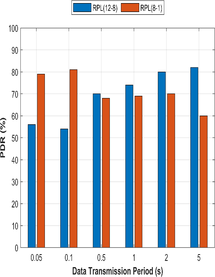
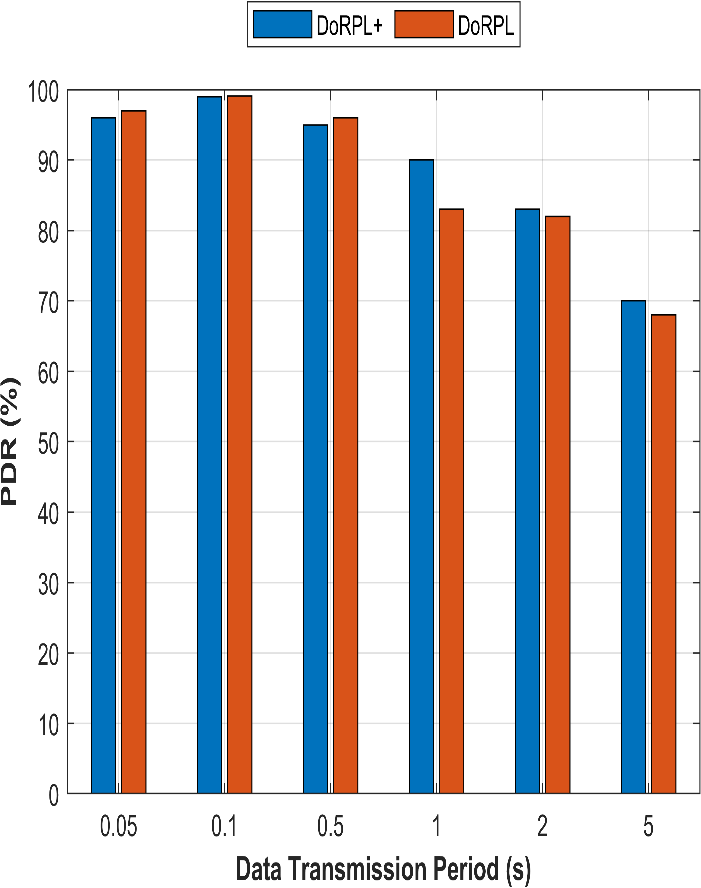
Figure 9: Evaluating Packet Delivery Ratio Across Varied Data Transmission Periods: (a) A Comparative Study with RPL, and (b) A Comparative Analysis of DoRPL Versus DoRPL+

The handoff delay in the node speed of RPL(12-8)routing is thoroughly depicted in Table 7 under various node speeds and data transmission intervals. The handoff delay shows a noticeable pattern at a rather slow node speed of 0.5 meters per second. The duration gradually increases to 25 seconds at a 5-second period, starting at 4.5 seconds for a 0.05-second transmission time. The delay values increase along with the node speed, reaching a peak of 24.5 seconds for a 5-second transmission period when the node speed is increased to 1 meter per second. Some oscillations in the delay values at 2 meters per second. For instance, the delay is 9 seconds with a transmission period of 0.5 seconds, but it increases to 18 seconds at a transmission time of 2 seconds. This shows that node speed and handoff delay in RPL(12-8) have a complex connection, with different speeds resulting in distinct delay profiles. These results highlight the need to carefully consider the interplay between node speed and transmission duration during network design and optimization.

Table 7: Analyzing Handoff Delay Variations in RPL Routing with Diverse Node Speeds

Table 8 offers a detailed analysis of handoff delay in the context of DoRPL routing, accounting for different node speeds and data transmission times. The handoff latency is very little when node speed is set to a modest 0.5 metres per second, ranging from 0.079 seconds at a 5-second transmission interval to 0.084 seconds at 0.05 seconds. The delay values remain continuously low, with a maximum of 0.09 seconds at a 0.05-second transmission period, when we increase the node speed to 1 metres per second. Similarly, DoRPL maintains a low handoff delay at 2 m/s, with values ranging from 0.081 to 0.09 seconds throughout various transmission intervals. According to this, DoRPL is resilient to changes in node speed, ensuring a short handoff delay across a range of network circumstances. These results highlight DoRPL routing’s effectiveness and dependability in practical settings.

Table 8: Exploring Handoff Delay Variability in DoRPL Routing Across Varying Node Speeds

In Table 9, describes an handoff delay within the domain of DoRPL+ routing, while considering diverse node speeds and transmission periods. At a relatively conservative node speed of 0.5 meters per second, the handoff delay remains consistently and impressively low at a mere 0.005 seconds, irrespective of the transmission period. By increase the node speed to 1 meter per second, the delay values maintain their efficiency, with only a marginal increase to 0.006 seconds at a 0.05-second transmission period. Even at a brisk node speed of 2 meters per second, DoRPL+ demonstrates remarkable stability, showcasing minimal handoff delays ranging from 0.004 to 0.084 seconds across various transmission periods. These findings underscore the robustness and adaptability of DoRPL+ routing in managing different node speeds, ensuring that handoff delays remain consistently minimal. Such performance is paramount for ensuring the seamless and dependable operation of communication networks, particularly in dynamic scenarios.

Table 9: Assessing Handoff Delay Across Various Node Speeds in DoRPL+ Routing

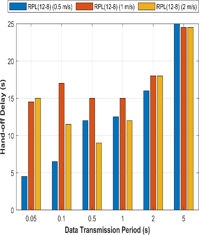
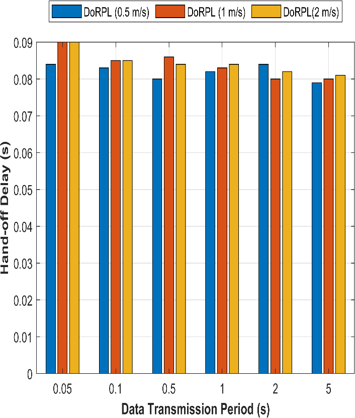
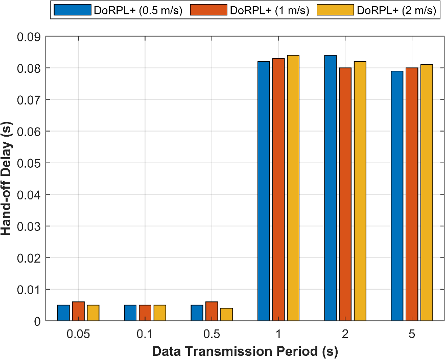
Figure 10: Hand off latency with various node speeds (a)RPL Routing (b) DoRPL routing (c) DoRPL+ Routing

In Table 10, we delve into a comprehensive analysis of packet delivery ratios within the realm of RPL routing, considering various node speeds and data transmission periods. At a node speed of 0.5 meters per second, the packet delivery ratio for RPL(12-8) exhibited strong performance, with values ranging from 68% at a 0.5-second transmission period to 81% at 0.1 seconds. When the node speed increased to 1 meter per second, the performance dynamics shifted, with a peak of 82% at a 5-second transmission period and a low of 54% at 0.1 seconds, and at a rapid 2 meters per second, there is more variability in delivery ratios, ranging from 30% to 79% across different transmission periods. These findings underscore the intricate relationship between node speed and packet delivery in RPL routing, highlighting the need for careful consideration of these factors in network design and optimization efforts.

Table 10: RPL routing packet delivery ratio at various node speeds

Table 11 provides an illustration of packet delivery ratios within the DoRPL routing, accounting for varying node speeds and data transmission periods. When the node speed is set at 0.5 meters per second, DoRPL consistently delivers impressive performance, with delivery ratios ranging from 98% at a 0.5-second transmission period to 99.7% at 0.1 seconds. As the node speed escalates to 1 meter per second, the performance remains robust, with a peak delivery ratio of 99.1% at 0.1 seconds and a gradual decline to 68% at 5 seconds. Even at a brisk 2 meters per second, DoRPL demonstrates resilience, maintaining delivery ratios within the range of 69% to 96% across various transmission periods. These results highlight the effectiveness of DoRPL routing in adapting to different node speeds, ensuring reliable packet delivery in diverse network scenarios.

Table 11: Packet delivery ratio with different node speed of DoRPL routing

Table 12 presents a analysis of packet delivery ratios in the DoRPL+ routing, accounting for varying node speeds and data transmission periods. At a node speed of 0.5 meters per second, DoRPL+ exhibits strong performance, with delivery ratios ranging from 92% at a 1-second transmission period to an impressive 99% at 0.5 seconds. Increasing the node speed to 1 meter per second maintains robust performance, with a peak delivery ratio of 99% at 0.1 seconds and a gradual decline to 70% at 5 seconds. When the node speed surges to 2 meters per second, DoRPL+ still maintains notable delivery ratios, with values spanning from 74% to 90% across different transmission periods. These findings highlight the adaptability of DoRPL+ routing in managing varying node speeds, ensuring reliable packet delivery in diverse network scenarios.

Table 12: Packet delivery ratio with different node speed of DoRPL+ routing

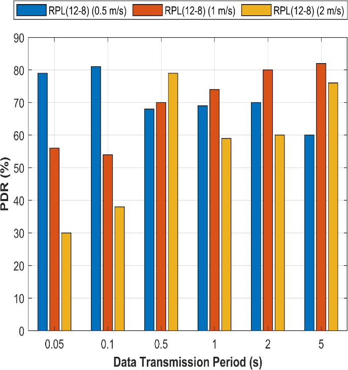
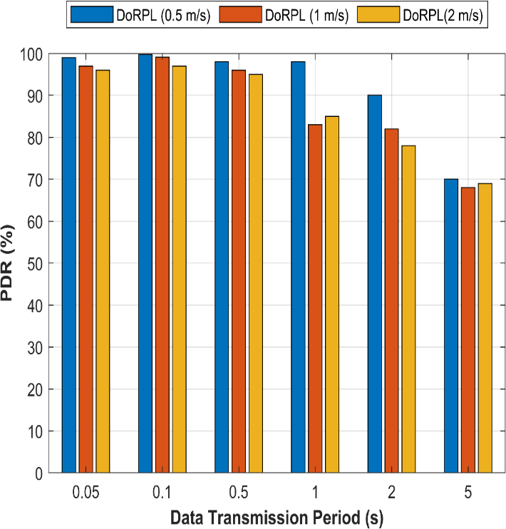
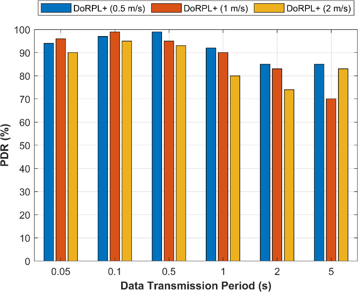
Figure 11: Ratio of packet delivery at various node speeds of (a ) RPL routing (b) DoRPL routing (c ) DoRPL+ Routing

Table 13 provides a comprehensive assessment of the total network overhead within the framework of RPL routing, accounting for different node speeds and data transmission periods. When the node speed is set at 0.5 meters per second, the network overhead exhibits varying values, ranging from 380 at a 5-second transmission period to 580 at 0.05 seconds. At a node speed of 1 meter per second, we observe a similar pattern, with overhead values fluctuating between 395 and 480 across different transmission periods. As the node speed increases to a brisk 2 meters per second, the network overhead remains dynamic, with values spanning from 388 to 490. These results underscore the intricate relationship between node speed and network overhead in RPL routing, emphasizing the need for careful consideration of these factors in optimizing network performance.

Table 13: Different node speeds and total network overhead in RPL routing

Table 14 presents a detailes evaluation of the total network overhead within the context of DoRPL routing, taking into account various node speeds and data transmission periods. When the node speed is set to a moderate 0.5 meters per second, the network overhead fluctuates, with values ranging from 400 at a 5-second transmission period to 643 at 0.5 seconds. At a node speed of 1 meter per second, the overhead remains dynamic, with values varying between 450 and 620 across different transmission periods. When node speed is further increased to 2 meters per second, the network overhead exhibits similar variability, ranging from 490 to 650. These findings highlight the influence of node speed on network overhead in DoRPL routing, emphasizing the importance of optimizing these parameters for efficient network performance.

Table 14: Total network overhead with varying node speeds in DoRPL routing

Table 15 provides a details of the total network overhead within the DoRPL+ routing, considering varying node speeds and data transmission periods. At a node speed of 0.5 meters per second, the network overhead exhibits some fluctuations, ranging from 500 at a 5-second transmission period to 610 at 0.05 seconds. Increasing the node speed to 1 meter per second maintains network overhead values in a similar range, with values varying from 505 to 612 across different transmission periods. When the node speed surges to 2 meters per second, the network overhead remains dynamic, spanning from 510 to 607. These results emphasize the intricate relationship between node speed and network overhead in DoRPL+ routing, highlighting the need for optimizing these parameters to enhance network efficiency.

Table 15: Total network overhead with different node speed in DoRPL+ routing

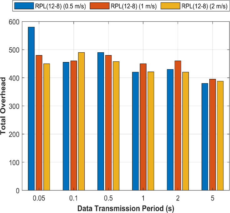
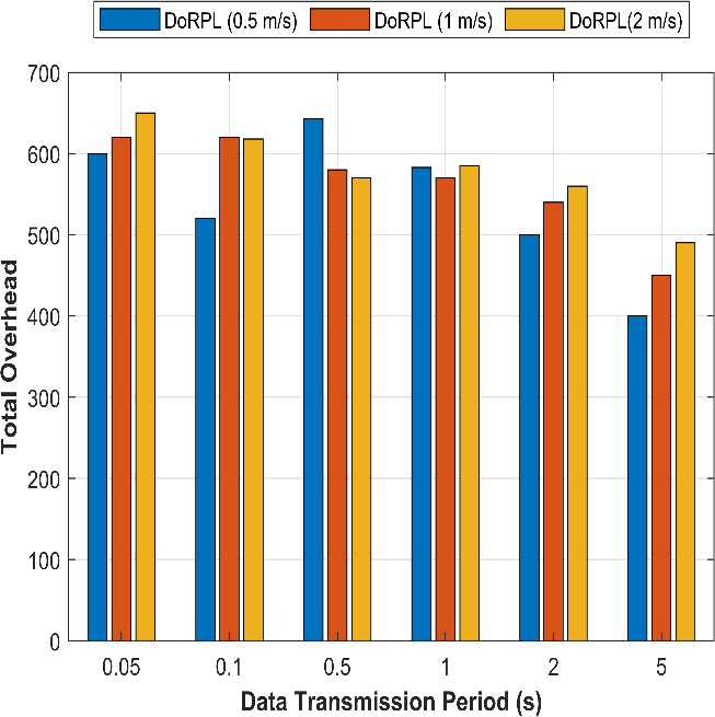
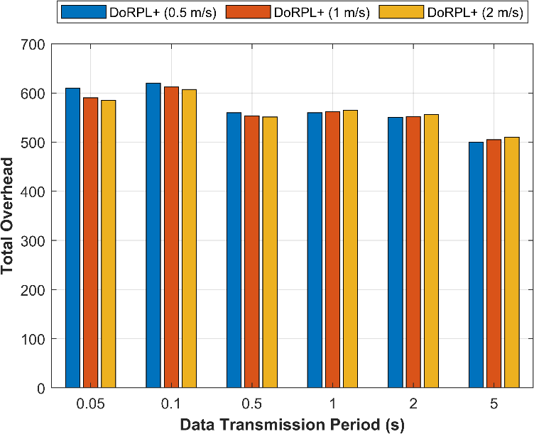
Figure 12: Total network overhead for nodes with various speeds (a) RPL (b) DoRPL (c) and DoRPL+

Table 16 offers a comparative analysis between DoRPL and different scenarios of DoRPL+ by varying the f variable, focusing on handoff delay. In the DoRPL column, as the f variable increases from 1 to 11, the handoff delay progressively decreases, ranging from 0.58 to 0.1. This demonstrates that as the value of f increases, indicating an extended interval for signal strength evaluation, DoRPL exhibits reduced handoff delay. These findings underscore the significance of parameter tuning in DoRPL and DoRPL+ protocols to optimize handoff performance in dynamic network environments.

Table 16: Comparison of DoRPL with various DoRPL+ Scenarios by changing the f variable’s handoff delay

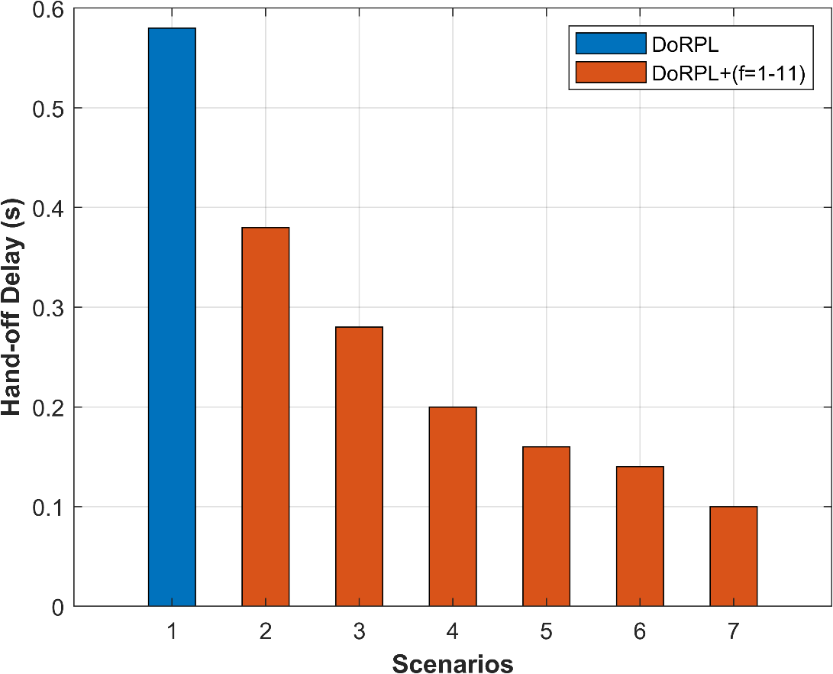
Figure 13 : comparing DoRPL with different DoRPL+ scenarios by altering the f variable’s Hand off delay

Conclusion

In conclusion, this innovative approach presents an advanced solution for enhancing mobility management in 5G-integrated RPL/6LoWPAN IoT networks. By employing a sophisticated hybrid deep learning framework, the proposed model effectively predicts and address link degradation and network conditions, enabling seamless soft hand-offs. The integration of the unique Savannah Fusion Optimization Algorithm (SFOA), combining African Vultures Optimization Algorithm (AVOA) and Whale Optimization Algorithm (WOA), further refines hand-off decisions. Additionally, for scenarios requiring more robust transitions, the method optimises backup parent node selection and initiates hard hand-offs when necessary. This comprehensive methodology also extends to multi-hop scenarios, where traffic load assessment and route selection are intelligently managed. This research marks a significant stride towards optimizing IoT network performance and reliability in the 5G era.

References

Verma, H., Chauhan, N., Chand, N. and Awasthi, L.K., 2022. Buffer-loss estimation to address congestion in 6LoWPAN based resource-restricted ‘Internet of Healthcare Things’ network. Computer Communications, 181, pp.236-256.

Wanasinghe, T.R., Gosine, R.G., James, L.A., Mann, G.K., De Silva, O. and Warrian, P.J., 2020. The internet of things in the oil and gas industry: a systematic review. IEEE Internet of Things Journal, 7(9), pp.8654-8673.

Thamilarasu, G. and Chawla, S., 2019. Towards deep-learning-driven intrusion detection for the internet of things. Sensors, 19(9), p.1977.

Son, V.Q. and Khoa, N.T.A., 2019, October. Evaluation of full-mesh networks for smart home applications. In 2019 International Symposium on Electrical and Electronics Engineering (ISEE) (pp. 73-78). IEEE.

Bouzebiba, H. and Lehsaini, M., 2020. FreeBW-RPL: a new RPL protocol objective function for internet of multimedia things. Wireless Personal Communications, 112, pp.1003-1023.

Safaei, B., Mohammadsalehi, A., Khoosani, K.T., Zarbaf, S., Monazzah, A.M.H., Samie, F., Bauer, L., Henkel, J. and Ejlali, A., 2020. Impacts of mobility models on RPL-based mobile IoT infrastructures: An evaluative comparison and survey. IEEE access, 8, pp.167779-167829.

Li, J., Niu, Y., Wu, H., Ai, B., Chen, S., Feng, Z., Zhong, Z. and Wang, N., 2022. Mobility support for millimeter wave communications: Opportunities and challenges. IEEE Communications Surveys & Tutorials, 24(3), pp.1816-1842.

Al-Kashoash, H., 2019. Congestion Control for 6LoWPAN Wireless Sensor Networks: Toward the Internet of Things.

Geetha, V., Bhat, A. and Thanmayee, S., 2022. New bit pattern based IPv6 address compression techniques for 6LoWPAN header compression. IEEE Access, 10, pp.80055-80070.

Miranda, C., Kaddoum, G., Boukhtouta, A., Madi, T. and Alameddine, H.A., 2022. Intrusion prevention scheme against rank attacks for software-defined low power IoT networks. IEEE Access, 10, pp.129970-129984.

Alsaeedy, A.A. and Chong, E.K., 2019. Mobility management for 5G IoT devices: Improving power consumption with lightweight signaling overhead. IEEE Internet of Things Journal, 6(5), pp.8237-8247.

Aljeri, N. and Boukerche, A., 2019. A two-tier machine learning-based handover management scheme for intelligent vehicular networks. Ad Hoc Networks, 94, p.101930.

Shakarami, A., Shahidinejad, A. and Ghobaei-Arani, M., 2021. An autonomous computation offloading strategy in Mobile Edge Computing: A deep learning-based hybrid approach. Journal of Network and Computer Applications, 178, p.102974.

Janiesch, Christian, Patrick Zschech, and Kai Heinrich. “Machine learning and deep learning.” Electronic Markets 31, no. 3 (2021): 685-695.

Rabet, I., Selvaraju, S.P., Adeli, M.H., Fotouhi, H., Balador, A., Vahabi, M., Alves, M. and Björkman, M., 2021, June. Pushing IoT mobility management to the edge: Granting RPL accurate localization and routing. In 2021 IEEE 7th World Forum on Internet of Things (WF-IoT) (pp. 338-343). IEEE.

Miranda, C., Kaddoum, G., Boukhtouta, A., Madi, T. and Alameddine, H.A., 2022. Intrusion prevention scheme against rank attacks for software-defined low power IoT networks. IEEE Access, 10, pp.129970-129984.

Alsukayti, I.S. and Singh, A., 2022. A lightweight scheme for mitigating RPL version number attacks in IoT networks. IEEE Access, 10, pp.111115-111133.

Manikannan, K. and Nagarajan, V., 2020. Optimized mobility management for RPL/6LoWPAN based IoT network architecture using the firefly algorithm. Microprocessors and Microsystems, 77, p.103193.

Samuel, C., Alvarez, B.M., Ribera, E.G., Ioulianou, P.P. and Vassilakis, V.G., 2020, July. Performance evaluation of a wormhole detection method using round-trip times and hop counts in RPL-based 6LoWPAN networks. In 2020 12th International Symposium on Communication Systems, Networks and Digital Signal Processing (CSNDSP) (pp. 1-6). IEEE.

Mbarek, B., Ge, M. and Pitner, T., 2021. Proactive trust classification for detection of replication attacks in 6LoWPAN-based IoT. Internet of Things, 16, p.100442.

Paul, A. and Pillai, A.S., 2021, September. A Review on RPL Objective Function Improvements for IoT Applications. In 2021 2nd International Conference on Advances in Computing, Communication, Embedded and Secure Systems (ACCESS) (pp. 80-85). IEEE.

Garg, S., Kaur, K., Kumar, N., Kaddoum, G., Zomaya, A.Y. and Ranjan, R., 2019. A hybrid deep learning-based model for anomaly detection in cloud datacenter networks. IEEE Transactions on Network and Service Management, 16(3), pp.924-935.

Pasikhani, A.M., Clark, J.A. and Gope, P., 2021, October. Reinforcement-Learning-based IDS for 6LoWPAN. In 2021 IEEE 20th International Conference on Trust, Security and Privacy in Computing and Communications (TrustCom) (pp. 1049-1060). IEEE.

Panda, N. and Supriya, M., 2023. Blackhole Attack Prediction in Wireless Sensor Networks Using Support Vector Machine. In Advances in Signal Processing, Embedded Systems and IoT: Proceedings of Seventh ICMEET-2022 (pp. 321-331). Singapore: Springer Nature Singapore.

Rabet, I., Selvaraju, S.P., Fotouhi, H., Alves, M., Vahabi, M., Balador, A. and Björkman, M., 2022. Sdmob: Sdn-based mobility management for iot networks. Journal of Sensor and Actuator Networks, 11(1), p.8.

Editorial Staff

Academic Master Education Team is a group of academic editors and subject specialists responsible for producing structured, research-backed essays across multiple disciplines. Each article is developed following Academic Master’s Editorial Policy and supported by credible academic references. The team ensures clarity, citation accuracy, and adherence to ethical academic writing standards

Content reviewed under Academic Master Editorial Policy.

• Editorial Staff

  Grid-Connected Solar PV Systems and Power Quality Review
• Editorial Staff

  Predicting Cardiovascular Diseases with PCA and Artificial Neural Networks
• Editorial Staff

  Maternal and Neonatal Outcomes Following Water Birth Systematic Review and Meta-Analysis
• Editorial Staff

  Electrospun Polymeric Nanofibers for Biomedical Applications