HED-Net for Energy Theft Detection in Power Grids

Abstract

Our research begins with a meticulous approach to data processing, starting with a thorough analysis and data cleaning. This includes handling missing values and outliers, employing K-nearest neighbours (KNN) imputation, and applying z-score normalization. Subsequently, we conduct data exploration and visualization (EDA) to gain deeper insights. In preparing the training and testing datasets, we introduce a novel hybrid data-splitting method. This approach combines traditional random splitting with a stratified strategy based on consumer profiles and geographical regions, ensuring a balanced representation of non-fraudulent and energy theft cases. Feature extraction plays a pivotal role, encompassing statistical metrics such as mean, standard deviation, skewness, and kurtosis, capturing essential aspects of electricity consumption patterns. We also introduce correlation-based features to measure relationships with external factors. The hybrid OPTIMIZATION is carried out by using the Orca Predation Algorithm (OPA) and Starling Murmuration Optimizer (SMO)Our unique contribution is the introduction of the Hybrid Enhanced Detection Network (HED-Net) for classification. HED-Net integrates a Temporal Convolutional Neural Network (TCNN) for temporal pattern extraction, a Spatial Attention Module (SAM) for spatial relationships, and a Temporal-Spatial Fusion (TSF) module for seamless feature integration. Leveraging transfer learning on extensive electricity consumption data, HED-Net significantly enhances precision in energy theft detection, offering a promising solution in this domain. The experimental values are reported as supplied; the evaluation limitations discussed below restrict their interpretation.

Keywords: Orca Predation Algorithm (OPA) and Starling Murmuration Optimizer (SMO);K-nearest neighbours; Hybrid Enhanced Detection Network; Temporal Convolutional Neural Network .

Introduction

With the strong growth of the global economy and the continuous development of data mining, enterprises pay more and more attention to and emphasize the retention of existing customer relationships to establish long-term cooperation, foster its stability in today’s booming market. On the other hand, customers’ expectations are not limited to obtaining the best products and services, they also need face-to-face personalized business, hoping to receive exactly what they request in a short time. Therefore, Customer Relationship Management (CRM) came into being and has been rapidly developed, widely used in retail, real estate, service and other industries [1]. In the customer relationship management system, customer classification as an important means of customer relationship management, its task is to mine the potential relationship between users, the user’s own characteristics of the intrinsic value, in this way, users can be valued and retained, especially customers can be classified to cope with different needs, behaviors and preferences of customers [2]. ID3 algorithm is applied to customer value segmentation of aviation market, and decision tree is used to analyze the characteristic data of passengers [3]. ID3 algorithm and cost-sensitivity learning mechanism to customer value segmentation and achieved ideal results. This theory reduces the pressure of storage space and is conducive to processing massive data [4]. Among many alternative clustering algorithms suitable for customer value analysis, K-means clustering is the most widely used [5].

On the basis of the net present value evaluation system, two indexes of sales volume and customer development potential are added to improve the value evaluation system, it makes up for the deficiency of the net present value evaluation system [6]. Profitability, image, barriers, stability and strategic alliance, the customer acquisition difficulty index is subdivided into four sub-indicators: Construction cost, marketing cost, degree of competition and customer response, and establish the telecom enterprise customer value evaluation index system [7]. The customer value evaluation system of telecom enterprises from three dimensions of customer current value, potential value and customer loyalty [8]. The customer value of individual customers so as to identify real high-value customers and formulate relevant management strategies [9]. Roughly divides the factors that drive customer value into three categories: Are respectively the characteristics related to the product, service and promotion. At the same time, some scholars are also doing research on the dynamic driving of customer value [10][11].

Comparative experiments assessed clustering accuracy, model effectiveness, e-commerce data distribution, and calculation times for various clustering algorithms, enhancing understanding [12]. A novel penthagorean fuzzy k-means approach emerges, utilizing the 5th power as a variant of q-rung orthopair fuzzy sets [13]. Employing the K-means clustering algorithm aids waste collection agencies in waste-dumped area tracking and route optimization by identifying clusters and highlighting attention-demanding routes [14]. Special focus was given to determining the optimal number of clusters using the elbow method and pseudo-F statistic [15].

The main Contribution of this research is as follows:

The data is collected through https://www.sciencedirect.com/science/article/pii/S2352484721006405

To analyse and preprocess of data, Data cleaning and KNN based imputation, Data normalization by zScore and Data is explored and visualized by eda is carried out.

To prepare for Training and Testing Dataset

Hybrid Data Splitting and Balancing are performed

To create the training and testing datasets, introduce a hybrid data-splitting technique

To extract the Feature, Statistical Features and Correlation-Based Features are introduced.

To select the feature selection–hybrid optimization is carried by using Orca Predation Algorithm (OPA) and Starling Murmuration Optimizer (SMO)

To classify the outcome Hybrid Enhanced Detection Network (HED-Net) based classification is used.

In this research structure, Section 1 serves as the introduction, and Section 2 defines an extensive literature review, surveying prior research. Section 3 details our innovative methodology. The last two sections, 4 and 5, present our research findings and facilitate an in-depth discussion, leading to a conclusive and impactful conclusion in Section 6.

Literature Review

In 2021, Aski et al. [16] have evaluated trust in individual web services using the nine mentioned criteria. Addressing web service selection’s significance, it analyzed the field. Findings displayed reasonable root mean square error (RMSE), precision, recall, and F-score values. In contrast to earlier studies, this research achieved reduced error levels and provided more accurate trust assessments for individual web services.

In 2020, Rosyadi et al. [17] have used to achieve a more comprehensive transition region, the transition region was amalgamated with k-means clustering. Initially, a grayscale image was simplified through k-means clustering, resulting in a lower variation of gray levels in a simplified image version compared to the original grayscale image.

In 2022, Raja et al. [18] have proposed a novel approach to enhance transition region extraction via merging with k-means clustering. Initially, k-means simplified the grayscale image into a lower gray level variation version. Two transition regions were then extracted: one from the original and another from the simplified image. Edge linking relied on Quasi-Euclidean distance, referencing the simplified image’s transition region.

In 2020, Laccetti and Lapegna et al. [19] have introduced a method for dynamically defining K’s value through optimizing a quality index, taking computational cost into account. Additionally, an approach to enhance algorithm performance and effectiveness was presented: a strategy for parallel implementation on contemporary multicore CPUs. This allowed for improved processing efficiency and resource utilization in the algorithm’s execution.

In 2015, Stevanović et al. [20] have introduced a novel and efficient method for quantifying and detecting distortion sources originating from the customer’s end. It relied on a modified power meter to measure distortion power, a non-linear load-only component of apparent power. Various definitions for calculating distortion power were examined, confirming the method’s viability.

In 2017, Kong et al. [21] have introduced a framework based on the latest and highly popular deep learning technique, the long short-term memory (LSTM) recurrent neural network (RNN), to address the complex issue. The framework was tested on real residential smart meter data and its performance was extensively compared to various benchmarks, including the field’s state-of-the-art load forecasting methods.

In 2016, Guo et al. [22] have introduced a two-stage approach for identifying power system dynamic signatures in real-time, employing phasor measurement unit (PMU) measurements and data mining. Typically, literature focused solely on predicting transient stability status for corrective control, neglecting generators’ dynamic behavior during instability events.

In 2016, Stein and Ramaseshan et al. [23] have used a qualitative research approach, employing a sequential incident technique to direct data collection. Inductive thematic analysis was applied to semi-structured interview transcripts gathered from customer narratives about retailer experiences. The findings revealed seven distinct elements of customer experience touchpoints: atmospheric, technological, communicative, process, employee-customer interaction, customer-customer interaction, and product interaction elements.

In 2017, So et al. [24] have explored how brand attractiveness influenced customer brand identification on the airline industry. Empirical testing of the conceptual model indicated significant indirect effects. Brand prestige, distinctiveness, and memorable experiences indirectly impacted customer brand identification through brand attractiveness. Additionally, brand social benefits had a direct contribution to this identification.

In 2016, Habibi et al. [25] have aimed to develop and estimate an extended model exploring customer-community relationships’ influence on perceptions and behaviors. It detailed how brand identification impacted interactions with community elements and markers, and consequently, brand relationship quality and loyalty. Employing a large sample and structural equation modelling, the research analyzed social media-based brand communities’ impact on brand relationship quality and loyalty.

Problem Statement

While the proposed method offers effective image segmentation through transition region and k-means clustering, its performance might degrade in cases where images have intricate textures or patterns. Additionally, selecting appropriate parameters for k-means clustering can be challenging and impact the segmentation accuracy, limiting its robustness across various image types [17]. Despite its performance improvement, the proposed approach for enhancing dynamic k-means algorithms through a parallel adaptive strategy on multicore CPUs may face limitations in terms of scalability. As the number of cores increases, managing the coordination of parallel processes and avoiding overhead might become more complex, potentially impacting the overall efficiency and speedup [19].

While the online identification of power system dynamic signatures using PMU measurements and data mining is promising, it may suffer from limitations in accurately predicting complex generator behaviors during instability events. The focus on transient stability status might overlook the intricate dynamics of generators and other components, affecting the reliability of the identification process in certain scenarios [22]. While testing an extended model of consumer behavior in the context of social media-based brand communities is valuable, it could potentially lack a comprehensive consideration of external factors that may influence consumer behavior beyond the scope of the model. External factors like broader cultural trends and economic shifts could impact consumer behavior in ways not fully captured by the extended model [25-26].

Proposed Methodology

In our proposed methodology, we initiate the process with a meticulous analysis and pre-processing of the collected data. This involves addressing missing values and outliers through data cleaning techniques, followed by K-nearest neighbors (KNN)-based imputation and z-score normalization. Subsequently, we delve into data exploration and visualization (EDA) to gain deeper insights. Moving on to the preparation of the training and testing datasets, we introduce a novel hybrid data-splitting approach. This method combines traditional random splitting with a stratified strategy based on consumer profiles and geographical regions, ensuring a balanced representation of both non-fraudulent and energy theft cases in each subset. Feature extraction is a crucial step, encompassing statistical features like mean, standard deviation, skewness, and kurtosis, which capture electricity consumption patterns’ essential aspects. Additionally, we introduce correlation-based features that measure relationships with external factors. Our unique contribution lies in the introduction of the Hybrid Enhanced Detection Network (HED-Net) for classification. HED-Net combines a Temporal Convolutional Neural Network (TCNN) for temporal pattern extraction, a Spatial Attention Module (SAM) for spatial relationships, and a Temporal-Spatial Fusion (TSF) module for effective feature integration. Leveraging transfer learning, HED-Net is pre-trained on extensive electricity consumption data, enhancing its precision in energy theft detection and it is depicted in Figure 1.

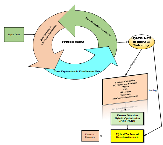
Figure 1: Overall Flow diagram of the proposed model

Analysis and pre-processing of data

Data collection

Data collection for this research was meticulously carried out by sourcing information from a reputable scholarly source, available at the following link: [https://www.sciencedirect.com/science/article/pii/S2352484721006405].

The dataset was procured with utmost care and attention to detail, ensuring its relevance and reliability for this research objective.

Data Pre-Processing

In the process of data mining, preparing the data is an important phase. It describes how data is prepared for analysis by cleaning, converting, and integrating it. Data preprocessing aims to enhance data quality and make it more appropriate for a certain data mining task.

Data Cleaning and Imputation

Data cleaning includes the following: (i) Fixing any errors in the data; and (ii) arranging the data in a way that would facilitate downstream analysis, for as by using clearer variable names, factor levels, and data transformation.

Data imputation is the process of replacing a realistically approximated value for a missing or faulty data item. The replacement value is meant to make further data analysis possible. To address missing values and outliers, we employ data-cleaning techniques.

K-nearest neighbors (KNN) BASED IMPUTATION

K-NN can be utilised as an imputation technique. The steps for using the K-NN approach are as follows:

Find the parameter K.

In this research, the variables K = 1,3,5,7 were used. In figuring out the K value for the K-NN approach, there is no set procedure. The level of accuracy in the classification will be reduced if the value of K is too small, but if it is too large, errors in restricting the value taken may also result, which will also have an indirect impact on accuracy.

Determine the Euclidian distance using Eq. (1) between instances of missing data and complete data.

D_(X,Y)=√(∑_J=1^S((X_J-Y_J)²)) (1)

As per Eq. (1) (X,Y) is the Euclidean distance, J is a data attribute with J=1, 2, 3, etc., and S is the data dimensions. Value from a J attribute with incomplete data, Value from another J-attribute with complete data.

The most minimal Euclidian distance is calculated using the distance information specified and the parameter K, which has been identified as the estimated value in the missing data. Eq. (2) applies Weight Mean Estimation to determine the value imputation.

X_J=(∑_K=1^k(W_KV_K))/(∑_K=1^k(W_K)) (2)

In which: Eq. (2) defines as Weight Mean Estimation, K: the number of parameters used with K=1, 2, 3, etc. Value K: nearest neighbor observation Based on the parameter k, K:value is the value of the full data on the attribute that includes the missing data.

Here, Eq. (3) is used to generate the formula for W_K.

W_K=(1)/(D_(X,Y)²) (3)

As per Eq. (3) Euclidian distance on each parameter of K is D_(X,Y). The research performed an analysis based on accuracy that was acquired by numerous classification methods in order to measure the estimated value of good or bad by imputation.

Data Normalization

The practise of rearranging data in a database so that users can use it for additional queries and analysis is referred to as data normalization. It is, in a nutshell, the process of creating clean data. Making the data appear consistent across all records and fields and removing unnecessary and unstructured data are two examples of how to do this.

z-SCORE

A statistical measurement known as the Z-score illustrates how closely a value relates to the mean of a group of values. The Z-score is determined using standard deviations from the mean. When a data point’s Z-score is 0, it means that it has the same score as the mean.

The following formula is used for to calculate the z-score

z=(x-μ)/(σ) (4)

As per Eq. (4) data point of interest is defined as x, to represent mean and standard deviation μ and σ is used.

Data Exploration and visualization

Data exploration is the first stage of data analysis, used to examine and visualise data in order to gain first insights or to spot potential areas or patterns for further investigation. Users may better see the big picture and discover insights more quickly by using interactive dashboards and point-and-click data exploration.

Data visualization is a method of displaying data using popular images like infographics, charts, and even animations. These informational visual representations convey intricate data relationships and data-driven insights in a way that is simple to understand.

Eda

Exploratory data analysis (EDA) is the process of examining and analysing record sets in order to understand their main characteristics, find patterns, find outliers, and find correlations between variables. EDA is typically performed as a first step before to more formal statistical research or modelling.

Hybrid Data Splitting and Balancing

A dataset is considered balanced if the number of input samples that reflect each output class (or target class) is equal. One of the methods listed below, such as oversampling or under sampling, can be used to achieve balance. size in class.

In an advanced method of processing datasets for machine learning, called hybrid data splitting and balancing, numerous strategies are combined to solve problems including class imbalance and data distribution. With this approach, training and testing sets are intended to be balanced in terms of class distribution and indicative of the real properties of the data. How hybrid data splitting and balancing functions is as follows:

Data Splitting

Stratified Sampling: The dataset is first divided into training and testing sets, with the goal of preserving the original data’s class distribution in each subset. By doing this, the ratio of various classes in the two sets is preserved.

Data Balancing

After the initial stratified split, additional balancing is applied to the training set exclusively. This involves random oversampling or under sampling. This may entail random under sampling (removal of certain samples from the majority class) or random oversampling (creation of additional copies of minority class samples).

Synthetic Data Generation: In some instances, synthetic examples for the minority class may be created using synthetic data generation techniques like SMOTE, improving its representation in the training set.

By combining these strategies, hybrid data splitting and balancing hopes to strike a balance between addressing class imbalance concerns (through oversampling, under sampling or synthetic data generation) and retaining the integrity of the dataset’s original distribution (by stratified sampling).

This hybrid technique is especially helpful when dealing with highly unbalanced datasets since it reduces the danger of overfitting or underperformance while keeping maintaining class proportions, which are crucial for model training and evaluation. In situations like fraud detection, medical diagnosis, and the prediction of uncommon events, it makes sure that machine learning models are reliable, fair, and accurate in their predictions.

Preparation of Training and Testing Dataset

Researchers propose a hybrid method of data splitting to produce the training and testing datasets. This method combines standard random splitting with a stratified approach based on customer characteristics and geographic areas. Our method lessens the detrimental impacts of class inequality by guaranteeing a balanced representation of both non-fraudulent and energy theft situations in each subgroup.

Feature Extraction

In this research, researchers incorporate statistical features such as average, standard deviation, skewness, and kurtosis into our research. These indicators give us important information about the intricacies of how people use electricity. Furthermore, they offer correlation-driven features that assess the relationships between consumption patterns and outside variables like weather and time-related aspects. By combining these correlation- and statistical-based components, our methodology deepens our understanding of consumption dynamics and the impact of outside factors, improving the accuracy and applicability of our findings for well-informed decision-making in energy-related contexts.

Statistical Features

Statistical features refer to important characteristics that are extracted from a dataset through careful statistical analysis. The basis of data science projects, these features act as the building blocks for research and analysis. Finding these statistical treasures is always our first priority when we start the path of dataset research. They include a variety of metrics that each provide a different viewpoint on the distribution, core trends, and variability of the dataset, including mean, variance, skewness, kurtosis, and others. These statistical inferences not only describe the data, but also set the stage for further analysis, modelling, and the extraction of useful inferences that support data-driven decision-making processes.

Mean

In statistics, in addition to the mode and median, the mean is one of the measures of central tendency. Simply put, the mean is the average of the values in the given set. It indicates that values in a particular data set are distributed equally. The three most frequently employed measures of central tendency are the mean, median, and mode.

As per the definition of the mean, it is calculated by the formula

x̅=(∑_I=1^N(x_I))/(n) (5)

According to the Eq. (5) n is the total number of given data and ∑(x_I) is the sum of all data values.

Standard deviation

The standard deviation is a metric that reveals how much variance from the mean there is, including spread, dispersion, and spread. A “typical” variation from the mean is shown by the standard deviation. Because it uses the data set’s original units of measurement, it is a well-liked measure of variability. When data points are closely spaced from the mean, there is a small variation, and when they are far spaced from the mean, there is a large variation. The standard deviation determines how much the values deviate from the mean. The most popular way to assess dispersion is standard deviation, which is based on all values. Therefore, even a small change in one value can modify the standard deviation’s value. Although it is independent of scale, it is not. Additionally, it helps with some complex statistical issues.

S=√((1)/(N-1)∑_I=1^N((X_I-X̅)²)) (6)

According to the Eq. (6) the Sample standard deviation is define as S, in sample number of observation is denoted as N, in sample the Ith observation is denoted as X_I and X̅ is the sample mean.

Skewness

A statistical metric known as skewness analyses the asymmetry of a probability distribution. It measures how much the data is moved to one side or skewed. A distribution with positive skewness has a longer tail on the right side, while one with negative skewness has a larger tail on the left. Skewness aids in comprehending a dataset’s form and outliers. There are many ways to calculate skewness, but Pearson’s coefficient is the one that is most frequently employed.

Pearsons first coefficient=(Mean-mode)/(Standard deviation) (7)

Kurtosis

A statistical term known as kurtosis characterises a probability distribution’s form. When compared to a normal distribution, it reveals information about the distribution’s tails and peaks. While negative kurtosis suggests lighter tails and a flatter distribution, positive kurtosis suggests heavier tails and a more peaked distribution.

β₂=((e(X)⁴)/((e(X)²)²))-3 (8)

The expected value of Xis mentioned as e

Correlation based Features

A specialized set of properties known as correlation-based features illustrates the connections between variables in a dataset. These features go beyond solitary data points to show how several variables interact with one another. They provide insightful information on dependencies, patterns, and cause-and-effect dynamics by quantifying the strength and direction of links. In data analysis, correlation-based features are especially important because they reveal hidden relationships between variables and help us comprehend how outside elements, such as the weather, the time of day, or user behaviour, affect the data of interest. Utilising these attributes can produce predictive models and better decisions across a range of industries, from healthcare to banking.

Feature Selection

In this research, the feature is selected by the hybrid optimization of combining Improved ORCA predation Algorithm and Starling Murmuration Optimizer (SMO) algorithm.

Hybrid Optimization- Improved Orca Predation Algorithm (OPA)

A) Orca Predation Algorithm

One of the most modern swarm intelligence systems, the orca predation algorithm (OPA), is important to distinguish it from other algorithms with similar names, such as the killer whale algorithm, ORCA optimization algorithm (OOA), orca’s algorithm (OA), and artificial orcas’ algorithm (AOA) (which all have lower annual citation counts, and some of them even have none at all), as well as from other programming structures that have nothing to do with optimization algorithms or biomimetics. The OPA follows killer whales’ (Orcinus orca’s) hunting techniques, intelligent animals on par with us. They hunt their prey in groups, using echolocation to locate it and sonar communication to communicate information and plan their attacks. They don’t base their attacks on a random feeding frenzy; instead, they are carefully organised and set up. Because of this, orcas are violent attackers that even hunt on sharks, making them the ocean’s top predators. The OPA was founded as a result of its hunters’ violent effectiveness.

The particulars are described below in more detail:

Initialization,

The chasing stage of an orca hunt,

When orcas hunt, they attack, and

Stop condition.

Initialization

When the orca group’s size and problem’s dimension are both set to N and D, respectively, in the OPA, the orca group’s mathematical expression is

x=[[X_1,1 , X_1,2 , ⋯ , X_1,d] ; [X_2,1 , X_2,2 , ⋯ , X_2,d] ; [⋯ , ⋯ , ⋯ , ⋯] ; [X_n,1 , X_n,2 , ⋯ , X_n,d]] (9)

where, by means of Equation (10), everyone is given a random initialization:

X_I,J=lb_J+(ub_J-lb_J)×rand (10)

where rand is a random number between [0, 1], ub represents the upper bound of the search space, and lb indicates the lower bound, and I = 1,2,…, n; J = 1,2,…, d.

The chasing phase or orca hunting

Orcas don’t just hunt in packs when they spot a pack of prey; they also interact and collaborate together through sonar. The prey will be pushed into a restricted area by orcas when they disperse and force them to the surface.

We divide the chase stage into two minor components based on this behavior: driving prey and surrounding prey. One of them gets selected at random by the orca to go hunting.

B) Driving prey

The orca must pursue its victim until it reaches the water’s surface. Even though there are few orcas, the search space is tiny, and the hunting terrain is straightforward, orcas are able to quickly and precisely locate their prey. To correctly get to the desired position, still is difficult. In order to keep the orca group from straying from the target at this time, it is also crucial to control the central position of the orca group in order to bring it near to the prey. Two tracking techniques were extracted and categorised based on the magnitude of the orca population. When the orca population is big (rand > q), we selected the first strategy.

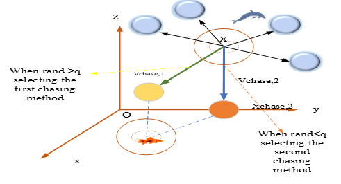
Figure 2: Driving Prey

For the movement speed and corresponding position of orcas during driving their prey, apply the formula below:

V_chase,1,I^T=A×(D×X_best^T-f×(B×m^T+C×X_I^T)) (11)

V_chase,2,I^T=e×X_best^T-X_I^T (12)

m=(∑_I=1ⁿ(X_I^T))/(n) (13)

C=1-B (14)

X_chase,1,I^T = X_I^T + V_chase,1,I ^Trand> Q, (15)

X_chase,2,I^T = X_I^T + V_chase,2,I^T rand≤ Q. (16)

When T denotes the number of iterations, V_chase,1,I^T denotes the ith orca’s chasing speed during time T after choosing the first chasing method, and V_chase,2,I^T has the same meaning. X_chase,1,I^T is the location of the ith orca after selecting the first chasing method during time T, and V_chase,2,I^T has the same meaning as M, which stands for the average position. e is a random number between [0,2], A,B,D,and Q are also random values, all of which are between [0,1], and f is 2. Among these, Q denotes the likelihood of selecting a particular chasing strategy. Q= 0.9 is the value at which OPA performs the best after numerous experiments.

Surrounding Prey

When orchestrating the ascent of their prey to the water’s surface, orcas employ a strategic formation. They create a maneuverable sphere around their target, facilitating efficient coordination. During this encirclement, orcas utilize sonar communication to exchange vital information with their fellow pod members. Calculations for their next movements hinge on the positions of three randomly chosen orcas within the group. These positional adjustments are critical in orchestrating successful hunts and exemplify the remarkable teamwork and intelligence displayed by these remarkable marine predators.

X_chase,3,i^T = X_J1,k^T+U×(X_J2,K^T-X_J3,K^T) (17)

U=2×(rand-1/2)×(Max_tier-1)/(Max_Tier) (18)

Max_Tier serves as the iteration limit, while j1, j2, and j3 refer to the distinct, randomly selected orcas within the population. The variable X_chase,3,i^Trepresents the position of the Ith orca following their selection of the third chasing method at timeT.

Orca placements should be adjusted.

`Orcas possess the ability to sense their prey’s location through sonar and adapt their positions accordingly. During the chase phase, if orcas detect their prey, they actively pursue and adjust their positions; otherwise, they maintain their original locations. The mathematical formula for updating positions is expressed as follows:

{X_chase,I^T = X_chase,I^T if f (X_chase,I^T) < f (X_I^T) ; X_chase,I^T = X_I^T if f (X_chase,I^T) ≥ f (X_I^T) (19)

where the fitness function value for X_chase,I^T is expressed by f (X_chase,I^T). The better position for addressing the smallest challenge is denoted by a fitness function value that is lower.

The hunting phase of orcas while attacking

C) Attacking the prey

During the prey attack phase, orcas exhibit a coordinated strategy. Four orcas are strategically positioned for optimal attacks, chosen to strike a balance between directional stability and convergence speed. Orcas taking their turn enter the prey enclosure, using tail slams to incapacitate the prey before consuming it. To maintain this formation, other individuals align their movements with the four attack orcas’ positions. When orcas return to replace others, they determine their direction based on nearby orcas. The attack stage involves calculating orcas’ movement speed and positions, a process encapsulated by the formula presented and depicted in Figure 2 of the model.

V_attack,1,I^T = (X₁^T + X₂^T + X₃^T + X₄^T) /4 – X_chase.Iʹ ^T (20)

V_attack,2,I^T =(X_chase,J1^T + X_chase,J2^T + X_chase,J3^T)/3-X_{I ʹ}^T (21)

Xattack,IT = Xchase,IT + G1× Vattack,1,IT + G2× Vattack,2,I‘T (22)

where J1, J2, and J3 are randomly selected orcas from the pack of N, V indicates speed, numbers 1 to 4 identify orcas in the optimal locations, and the subscript attack means the value is right for the attacking stage. The parameter G₁is a number created at random between [0, 2], while the parameter G₂is a number generated at random between [2.5, 2.5]. Figure 3 as Shown in below.

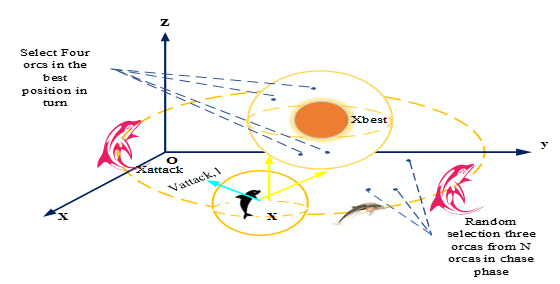
Figure 3: Attacking Prey

Adjust the positions of ORCA

In the attack phase, like the chase process, orcas rely on sonar to detect prey and fine-tune their positions accordingly. When an orca captures its prey, it navigates to the boundary of the fish’s range and delivers a decisive strike to obtain food. Additionally, to account for potential strandings, a constant p₂ is introduced. If a randomly generated number falls below p₂, the orca’s position is determined by lb (presumably another parameter or factor).

Stop condition

Until the stop condition is met, the algorithm repeatedly surrounds, drives, and attacks prey

D) Improved ORCA predation algorithm

The Improved Orca Population Algorithm (IOPA) incorporates a strategy-based Deep Learning (DL) approach to enhance orca individuals’ positioning within the population. In each iteration, two new candidates emerge: one through the original algorithm’s mechanism and the second via the newly introduced DL strategy. Orcas then update their positions based on their fitness. DL strategy creates distinct neighbourhoods for each orca, enabling mutual learning. This updated DL approach bolsters population diversity, reduces the risk of local optima, and accelerates algorithm convergence. See below for further specifics.

Dimension Learning

The DL strategy in the Innovative Orca Population Algorithm calculates individual neighbourhood radii based on inter-iteration information. It derives dimension groups for each individual using these radii and the current group. Subsequently, dimension-specific individuals are computed through this dimension group and the current group. This approach harnesses the best experiences of individuals to consolidate high-quality dimensional information from the group’s best experiences. DL establishes an independent learning paradigm for each orca, learning from the optimal positions in each dimension. This autonomous learning bolsters group diversity and mitigates the risk of local optima. After DL implementation, it compares the DL population with the original algorithm’s iteration population, selecting superior individuals based on a specific formula to update the orca population.

Rad_I^T=∥X_I^T-X_I^T-1∥ (23)

where X_I^T is the position of the ith person in the Tth iteration, Rad is the neighbourhood radius, and the same logic is denoted by X_I^T-1.

NE_I^T={X_J^T|d(X_I^T,X_J^T)≤Rad_I^T,X_J^Tϵpopulation } (24)

where d represents the distance and NE_I^T denotes the area around the Ith person in the Tth iteration.

X_I-Dl,J^T=X_I,J^T+(X_ne,J^T-X_R,J^T) (25)

where X_I-Dl,J^T denotes the new individual created using the DL method, X_ne^Tdenotes the individual is randomly chosen from the neighborhood NE_I^T, and X_R^T denotes the population randomly selected.

X_I^T={X_I^T, if f(X_I^T)<f(X_I-DL^T) ; X_I-DL^T, if f(X_I^T)<f(X_I-DL^T) (26)

Opposition based Learning

The IOPA algorithm enhances iteration population diversity via OP, boosting exploration and the OPA algorithm’s convergence speed.

X̅_I,J=ub_J+lb_J-X_I,J (27)

The OP strategy calculates an individual’s opposite position based on their current location and the space’s defined range. In a 1D space, it mirrors the point symmetrically. In a 2D space, represented with red and blue stars denoting opposite positions, it enhances algorithm exploration and population diversity. Once the candidate solution’s opposed position, xi, is established, population updating occurs using a greedy strategy as follows.

X_I^T={X_I^T, if f(X_I^T)<f(X̅_I^T) ; X̅_I, if f(X_I^T)<f(X̅_I) (28)

Starling Murmuration Optimizer (SMO)

When huge groups of numerous birds fly and spin in carefully linked shape-shifting living clouds, generating wonderful visual spectacles, this occurrence is known as starling murmuration (family Sturnidae). The reason that behaviors is used in optimization is because none of the vast numbers of birds flying in unison ever crash with one another. It is hardly surprising that one of the SMO algorithm’s earliest real-world uses was to coordinate the flying of large swarm of drone.

The starling murmuration optimizer (SMO) is a metaheuristic algorithm introduced in 2022 by Zamani et al. It is a population-based algorithm utilizing a dynamic multi-flock construction. It introduces three new search strategies: separating, diving and whirling.

Individual starlings are randomly dispersed during the algorithm’s first phase. The following equation describes the initial location of the ith starling in the group of N birds:

x_id = x_d^l+ rand (0,1) (x_d^u – x_d^l), i = 1,2, ⋯N; d = 1,2, ⋯D, (29)

Where N is the whole starling population, D is the number of dimensions there are in the search space, x_id is the starling’s dth dimension. S_i, x_d^u the search space’s upper bound and x_d^l is the search space’s lowest bound. A random function with a value between 0 and 1 is called rand (0, 1).

Following setup, a few of the starlings split off from the flock to create a new flock called Psep, which will scour the area in line with

P_sep = (log((t+D)))/(2log((t_max))) , (30)

where t denotes the current iteration and tmax denotes the maximum number of iterations allowed. The search plan is established by

X_i(t+1) = X_G (t) + Ξ₁ (y) [X_r, (u) – X_r (t)], (31)

where X_r‘(t) is the location chosen from a section of the fittest starlings and the separated flock, X_r(t) is a random selection from a population, and X_G(t) is the global position gained during iterative step t. A novel operator called the separation operator Ξ₁ (y) is based on the conventional quantum harmonic oscillator, where y stands for a random number drawn from the Gaussian distribution

The birds of prey that remain after the separation create the multi-flock, which has members f₁, f₂,…, f_k. dynamically. The qth flock’s quality Q_q(t) is determined by

Q_q(t) = (∑_i=1^k( ∑_j=1ⁿ(sf_ij (t))))/((1)/(n) ∑_i=1 ⁿ(sf_qi) (t)) (32)

must decide between the spinning (exploitation) or diving (exploration) search method. The rotating approach takes advantage of the vicinity of potential regions using a novel cohesion force operator, while the diving strategy uses a new quantum random diving operator to explore the search space. Here sf_ij(t) is the starling’s fitness score from the jth flock, f_j, and k is the murmuration’s M maximum number of flocks. The letter μ_q stands for the flocks overall average quality.

Hybrid Enhanced Detection Network (HED-Net) Based Classification

For classification, we introduce a cutting-edge deep learning architecture called “Hybrid Enhanced Detection Network (HED-Net).” HED-Net comprises three interconnected components:

Temporal Convolutional Neural Network (TCNN): This component specializes in capturing temporal patterns in electricity consumption data over different time intervals. It employs dilated convolutions and residual connections to extract intricate features.

TCNs are a specific kind of convolutional neural network that are well suited to handle time series because of its unique nature. TCNs adhere to two key principles: they prevent information from the future from leaking into the past by utilising causal convolutions, and their output has the same length as their input sequence (similar to LSTM networks). Causal convolution varies from normal convolution in that it does not use future values as inputs while obtaining the output at time T. This indicates that, given a kernel size K, the values of x_T-(K-1),x_T-(K-2), ………x_T-1,x_T are used to calculate the output o_T in the following figure 4.

To keep each layer at the same length as the input sequence, zero-padding of length k1 is applied. TCNs further use one-dimensional dilated convolutions in order to capture longer-term patterns. Because no pooling procedures are used in this convolution, there is no loss of resolution. It simply expands the network’s receptive field. In order to achieve dilation, as values are skipped between the convolutional operation’s inputs. Following is an example of how to formulate the full dilated causal convolution process over subsequent layers:

X_L^T=G(∑_K=1^k-1(W_L^KX_(L-1)^(T-(K×D))+B_L))) (33)

where W_L^K stands for the weight of position (K), X_L^Tis the output of the neuron at position (T) in the L-th layer, k is the width of the convolutional kernel, D is the dilation factor of the convolution, and B_L is the bias term. As an activation function, Rectified Linear Units (ReLU) layers are utilised (G(X)=max(0,X))Concatenating numerous TCN blocks is another typical method for expanding the network’s receptive field, as seen in the following Fig 4. However, this results in more complex designs with a greater number of factors, which makes the learning process more difficult. For this reason, each TCN block’s output is given a residual connection. Residual connections, which involve multiplying a TCN block’s input by its output (O=G(X+f(X)))were proposed by to enhance performance in very deep systems.

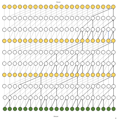
Figure 4: Temporal Convolutional Neural Network

TCNs are an effective deep-learning architecture for issues involving complex time series because of all these features. The primary benefit of TCNs is that, like RNNs, they can accommodate inputs of varying lengths by swiping the one-dimensional causal convolutional kernel. Due to their shared convolution architecture, which enables them to analyze lengthy sequences in parallel, TCNs are also more memory efficient than recurrent networks. The sequential processing of the input sequences by RNNs increases the computation time. TCNs are also trained using the conventional backpropagation technique, which avoids the gradient issues associated with the backpropagation-through-time algorithm (BPTT) used in RNNs.

Spatial Attention Module (SAM)

SAM focuses on spatial relationships between consumers, taking into account geographical factors and consumer interactions. It uses attention mechanisms to weigh the importance of different regions in the grid. Convolutional neural networks have a module for spatial attention called a spatial attention module. By utilising the spatial relationships between features, it creates a spatial attention map. In contrast to channel attention, which concentrates on what is informative, spatial attention concentrates on where information is. We initially perform average-pooling and max-pooling operations along the channel axis and concatenate them to produce an effective feature descriptor before computing the spatial attention. Then apply a convolution layer to the concatenated feature descriptor to create a spatial attention map m_S(f)ϵR^h×w that specifies where to emphasise or conceal.

By combining the channel information from two pooling procedures, researchers may create two 2D maps: f_avg^SϵR^1×h×wand f_max^SϵR^1×h×w. Each indicates the channel’s maximum and average-pooled features. The 2D spatial attention map is created by concatenating and convolving those with a regular convolution layer. The computation of the spatial attention is, in brief in Figure 5:

m_S(f)=σ[f^7×7[[AvgPool(f);MaxPool(f)]]] (34)

m_S(f)=σ[f^7×7[[f_avg^S;f_max^S]]] (35)

where σ signifies a convolution operation with a filter size of 7 x 7and indicates the sigmoid function f^7×7.

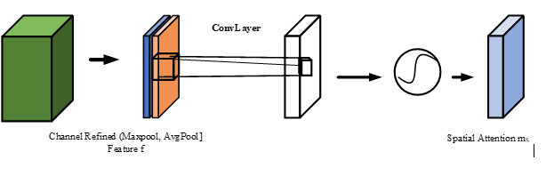
Figure 5: Spatial Attention Module

Cross Attention

To obtain hidden spatio-temporal representations, we process the multi-layered temporal input x_T-τϵx_Tinput in parallel through a multi-graph feature set denoted as θ.

The resulting representations, H, consist of elements

H={h_t-τ^θϵR^u|θϵ(x_w,x_p,x_S)τϵt_H} (36)

Where h_t-τ^θϵH, where θ ranges over the sets x_w,x_p,x_Sand τ belongs to the temporal set 𝑇ℎ. The superscript θ signifies spatial correlation information, while the subscript t-τ denotes temporal correlation information. To effectively combine spatio-temporal details, we employ a two-step spatio-temporal attention mechanism, as visually depicted in the following Figure 6.

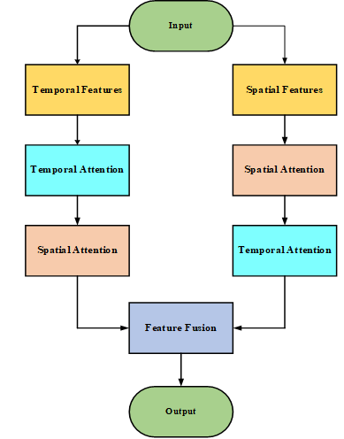
Figure 6: Flowchart for Cross Attention

This approach enhances our model’s ability to integrate and leverage both spatial and temporal information for a more comprehensive analysis.

Feature Fusion

The first step in our feature fusion procedure is splitting the spatio-temporal representation, abbreviated as h_T-τ^θ, into two different expression forms:

Here, we divide the data based on the same temporal instance but various spatial locations, yielding three distinct representations: h_T^x_W , h_T^x_P, and h_T^x_S. These depictions capture the spatial properties built into our heterogeneous multi-graphs. In this context, we group the data based on the same spatial location but various temporal instances, leading to three separate representations: h_T-R^θ, h_T-D^θ, and h_T-W^θ .These depictions incorporate multiple levels of temporal elements, which accurately captures how our data has changed throughout time.

{α^LS=softmax(h_T-τ^θw_h^LS+g^θw_g^LS+B^LS) ; h_T-τ^(s)=∑_θⁿ(α_θ^LS∙h_T-τ’^θ) h_T-τ^(s)ϵh^(s) (37)

{α^LT=softmax(h_T-τ^θw_h^LT+m_T-τw_m^LT+B^LT) ; h_θ^(T)=∑_τ^t_H(α_τ^LT∙h_T-τ’^θ) h_θ^(T)ϵh^(T) (38)

w_h^LT, w_m^LT, w_h^LS, and w_g^LS are trainable parameters. B^LT and B^LS are deviation vectors. m_T-τ stands for the density of the time slice H_t-τand g^θ stands for a compact vector of the graph.

In the second phase of our feature fusion process, illustrated in Figure 8, we build upon the outcomes of the first step, where we initially established a set of temporal attention. This initial step resulted in the creation of a spatial set that integrates temporal information, denoted as H^(t), comprising elements H^(t)={h_θ^(t)|θϵ(x_W,x_P,x_S)}Concurrently, spatial attention led to the formation of a temporal set containing spatial information, H^(S)denoted as H^(S)={h_T-τ^(S)|τϵt_H}

To progress further, we employ a cross-attention mechanism. This entails applying temporal attention to the newly fused spatial set, H^(S), and simultaneously performing spatial attention on the newly fused temporal set, H^(t). Through this intricate process, we derive a novel set of equations that encapsulate the interplay of spatio-temporal information, allowing us to glean deeper insights and patterns from our data. This step enhances the comprehensiveness of our feature fusion, paving the way for a more refined understanding of the complex dynamics within our dataset.

{α^2s=softmax(h_θ^(s)w_h^2s+g^θw_g^2S+B^2S) ; h^(ts)=∑_θⁿ(α_θ^2S∙h_θ^(t)) (39)

{α^2T=softmax(h_T-τ^(s)w_h^2T+m_T-τw_m^2T+B^2T) ; h^(st)=∑_τ^t_H(α_τ^2T∙h_T-τ^(s)) (40)

The notation employed here bears a resemblance to the formula notation used in the initial step. The essence of the cross-attention mechanism fusion lies in its ability to concurrently represent multi-layer temporal correlations and heterogeneous spatial correlations as two distinct perspectives, ultimately integrating them through cross-fusion.

In Equations (28) and (30), we observe the compression of H^(S) into h^(st) based on spatial continuity, capturing the essential spatial information. Conversely, Eqs (38) and (40) condense H^(t) into h^(ts) by emphasizing temporal continuity, reflecting the multi-level temporal features. The final step in this fusion process involves feeding these two compressed matrices into a fully connected layer to obtain the ultimate prediction result, expressed as:

x_T̂=tanh⁡(h^(ts)w_ts+h^(st)w_st+B ) (41)

In this equation, w_ts and w_st represent trainable parameters, while B accounts for bias. This fusion approach consolidates the temporal and spatial aspects of our data, culminating in a refined prediction outcome that reflects the intricate interplay between these vital dimensions.

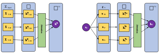
Figure 7: (a) Time Series-Temporal Fusion (b) Multigraph-Spatial Fusion

The basic components of our model are the spatial attention and temporal attention, which are expressed through Equations (28) and (29), respectively and it is shown in Figure 7., serve as the basic pillars of our feature fusion strategy. These attentions enable a more nuanced and thorough comprehension of the underlying spatio-temporal patterns by allowing us to concentrate on particular elements of the data. HED-Net leverages the power of transfer learning by pre-training on a vast dataset of electricity consumption patterns, enhancing its ability to generalize and detect energy theft accurately.

Result And Discussion

The table and plots retain the reported results. Under a common binary evaluation, accuracy is a weighted average of sensitivity and specificity; the reported accuracy of 0.997 exceeds both the reported sensitivity of 0.962 and specificity of 0.996. The false-positive rate of 0.007 and false-negative rate of 0.05 also do not complement the corresponding specificity and sensitivity. A different averaging scheme or evaluation split might explain some differences, but neither is sufficiently documented. Independent verification requires the labeled evaluation records and metric computation protocol.

Experimental Setup

In this research, this section explains about the implementation of the MATLAB in the proposed, alongside a comparison with other models, all aimed at achieving heightened accuracy in the Detection Network for Accurate Energy Theft Detection within Power Grids. Our assessment is underpinned by an array of vital metrics, including Sensitivity, Specificity, Accuracy, Precision, Recall, F-Measure, Negative Predictive Value (NPV), False Positive Rate (FPR), False Negative Rate (FNR), and Matthews Correlation Coefficient (MCC).

Overall performance analysis

From Table 1, the proposed model emerges, with an impressive Sensitivity score of 0.962, denoting its proficiency in accurately identifying energy theft incidents. Coupled with a Specificity of 0.996, it excels at distinguishing non-fraudulent cases, culminating in an outstanding overall Accuracy of 0.997. Moreover, its Precision at 0.966 underscores its capability to differentiate genuine energy theft from false alarms, while Recall, at 0.961, showcases its ability to retrieve pertinent instances. The F-Measure, balancing Precision and Recall, stands at 0.965, affirming the model’s robust performance. Our proposed model also demonstrates a strong NPV of 0.985, effectively minimizing the occurrence of false negatives. Furthermore, its low FPR at 0.007 and FNR at 0.05 signify its reliability in classification tasks. With an impressive MCC of 0.953, our proposed model stands as the optimal choice among the models considered, affirming its effectiveness in precise energy theft detection within power grids. In comparison, alternative models like LSTM, RNN, CNN, and MLP exhibit varying degrees of performance, with our proposed model consistently leading in Sensitivity, Specificity, Accuracy, and MCC, thus solidifying its suitability for this critical application.

Table 1: Overall Performance of the proposed model

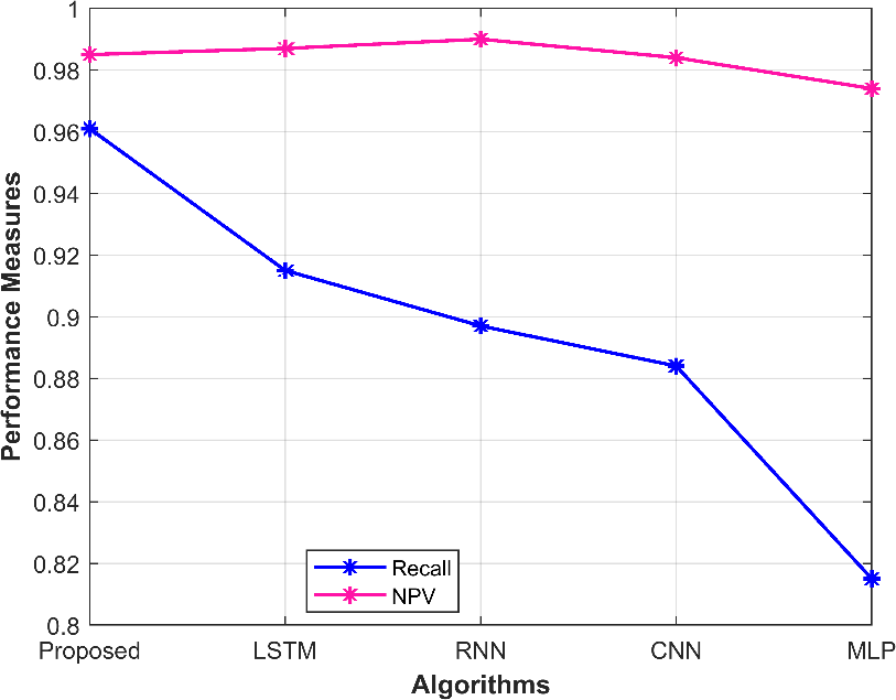
Figure 8: Graphical representation of the performance measures -Recall, NPV

From Figure 8 it is illustrates as that the proposed model’s performance measures Recall is higher than that of the other comparative models and at the same time the NPV value of the proposed model is lower than the sum of the other models.

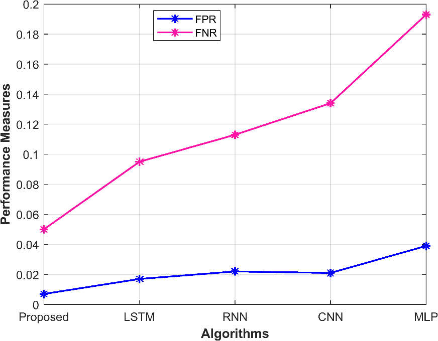
Figure 9: Graphical representation of the performance metrics-FPR and FNR

Figure 9 illustrates that the performance measures of the proposed models FPR and FNR are very lower than the other comparative models like LSTM, RNN, CNN and MLP.

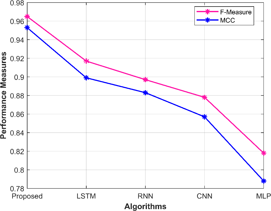
Figure 10: Graphical representation of the performance metrics-F-Measure and MCC

Figure 10 illustrates that the performance measures of the proposed models F-Measure and MCC are very higher than the other comparative models like LSTM, RNN, CNN and MLP.

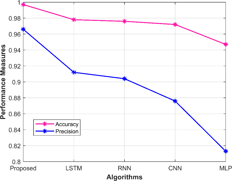
Figure 11: Graphical representation of the performance metrics-Accuracy and Precision

Figure 11 illustrates that the performance measures of the proposed models Accuracy and Precision are very higher than the other comparative models like LSTM, RNN, CNN and MLP.

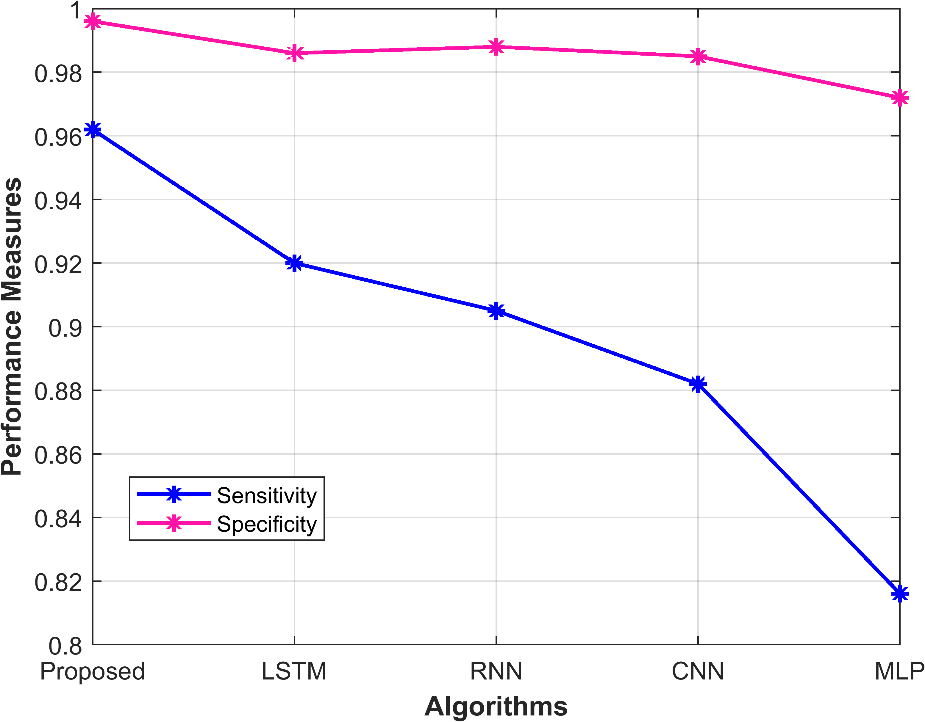
Figure 12: Graphical representation of the performance metrics-Sensitivity and Specificity

Figure 12 illustrates that the performance measures of the proposed models Sensitivity and Specificity are very higher than the other comparative models like LSTM, RNN, CNN and MLP.

Conclusion

In conclusion, this research presents a comprehensive approach for accurate energy theft detection in power grids through a Hybrid Enhanced Detection Network (HED-Net). We meticulously carried out the data collection and preprocessing, addressing missing values and outliers using techniques such as K-nearest neighbors (KNN) imputation and z-score normalization. Our data exploration and visualization (EDA) provided valuable insights. To ensure robust training and testing datasets, we introduced a hybrid data splitting technique, combining Improved ORCA predation Algorithm and Starling Murmuration Optimizer (SMO) algorithm which balanced non-fraudulent and energy theft cases, mitigating class imbalance issues. The feature extraction phase incorporated statistical and correlation-based features, enriching the model’s understanding of electricity consumption patterns. The heart of our approach, HED-Net, is a state-of-the-art deep learning architecture, comprising the Temporal Convolutional Neural Network (TCNN), Spatial Attention Module (SAM), and Temporal-Spatial Fusion (TSF). These components capture temporal and spatial patterns, leveraging transfer learning to enhance detection accuracy. In summary, our hybrid approach showcases promising results in energy theft detection, outperforming traditional models. By integrating data preprocessing, balanced dataset creation, and a cutting-edge deep learning network, we pave the way for more reliable and efficient energy theft detection in power grids. This research contributes significantly to improving the security and stability of energy distribution systems.

References

[1] Wu, J., Shi, L., Lin, W. P., Tsai, S. B., & Xu, G. (2020). An empirical study on customer segmentation by purchase behaviors using a rfm model and k-means algorithm. Mathematical Problems in Engineering, 2020(6), 1-7.

[2] RG Martínez, Carrasco, R. A., Garcia-Madariaga, J., Gallego, C. P., & Herrera-Viedma, E. (2020). A comparison between fuzzy linguistic rfm model and traditional rfm model applied to campaign management. case study of retail business. Procedia Computer Science, 162, 281-289.

[3] Jiao, N., Wang, F., & You, H. (2020). A new rd.-rfm stereo geolocation model for 3d geo-information reconstruction of sar-optical satellite image pairs. IEEE Access, 8, 94654-94664.

[4] Zong, Y., & Xing, H. (2021). Customer stratification theory and value evaluation-analysis based on improved rfm model. Journal of Intelligent & Fuzzy Systems: Applications in Engineering and Technology (40-3).

[5] Wei, J. T., Lin, S. Y., Yang, Y. Z., & Wu, H. H. (2020). Using a combination of rfm model and cluster analysis to analyze customers’ values of a veterinary hospital. IAENG International journal of computer science (47-3 Pt.1).

[6] Li, N., Jin, X., & Li, Y. (2020). Identification of key customer requirements based on online reviews. Journal of Intelligent and Fuzzy Systems, 39(1984), 1-14.

[7] Watada, J., Roy, A., & Vasant, P… (2020). Preference identification based on big data mining for customer responsibility management. International Journal of Intelligent Technologies and Applied Statistics, 13(1), 1-24.

[8] Li, J., & Cao, S… (2021). The study on high-value user identification of localized information platform. Journal of Physics: Conference Series, 1883(1), 012109 (8pp).

[9] Andre, H., Ghozal, M., Fitrilina, Baharuddin, & Asriyadi. (2021). Optimization signal quality on cellular network based on tilting-antenna. IOP Conference Series Materials Science and Engineering, 1041(1), 012010.

[10] Witek, M., & Uilhoorn, F. E. (2021). Influence of gas transmission network failure on security of supply. Journal of Natural Gas Science and Engineering (1), 103877.

[11] Ayta, E. (2020). Unsupervised learning approach in defining the similarity of catchments: hydrological response unit-based k-means clustering, a demonstration on western black sea region of turkey. International Soil and Water Conservation Research, 8(3), 321-331.

[12] Pan, H., Lei, Y., & Yin, S. (2021). K-means clustering algorithm for data distribution in cloud computing environment. International journal of grid and utility computing (12-3).

[13] Haktanir, E… (2021). A fuzzy film rating system using penthagorean fuzzy k-means clustering. Journal of multiple-valued logic and soft computing (37-5/6).

[14] Resmi, N. G., Shajan, A., Jose, J., George, J. P., & Harikrishnan, M. (2021). Solid waste tracking and route optimization using geotagging and k-means clustering. International Journal of Applied Engineering Research (8), 16.

[15] Warchalska-Troll, A., & Warchalski, T… (2022). The selection of areas for case study research in socio-economic geography with the application of k-means clustering. Wiadomosci Statystyczne (67-2).

[16] Aski, B. S., Haghighat, A. T., & Mohsenzadeh, M… (2021). Evaluating single web service trust employing a three-level neuro-fuzzy system considering k-means clustering. Journal of Intelligent & Fuzzy Systems: Applications in Engineering and Technology (40-5).

[17] Rosyadi, A. W., & Suciati, N. (2020). Image segmentation using transition region and k-means clustering. IAENG International journal of computer science, 47(1), 47-55.

[18] Raja, D. R. K., Kumar, G. H., Basha, S. M., & Ahmed, S. T. (2022). Recommendations based on integrated matrix time decomposition and clustering optimization. International Journal of Performability Engineering (18-4).

[19] Laccetti, G., Lapegna, M., Mele, V., Romano, D., & Szustak, L. (2020). Performance enhancement of a dynamic k-means algorithm through a parallel adaptive strategy on multicore cpus. Journal of Parallel and Distributed Computing (145-), 145.

[20] Stevanović, D. and Petković, P., 2015. A single-point method for identification sources of harmonic pollution applicable to standard power meters. Electrical Engineering, 97, pp.165-174.

[21] Kong, W., Dong, Z.Y., Jia, Y., Hill, D.J., Xu, Y. and Zhang, Y., 2017. Short-term residential load forecasting based on LSTM recurrent neural network. IEEE transactions on smart grid, 10(1), pp.841-851.

[22] T. Guo and J. V. Milanović, “Online Identification of Power System Dynamic Signature Using PMU Measurements and Data Mining,” in IEEE Transactions on Power Systems, vol. 31, no. 3, pp. 1760-1768, May 2016, doi: 10.1109/TPWRS.2015.2453424.

[23] Stein, A. and Ramaseshan, B., 2016. Towards the identification of customer experience touch point elements. Journal of Retailing and Consumer Services, 30, pp.8-19.

[24] So, K.K.F., King, C., Hudson, S. and Meng, F., 2017. The missing link in building customer brand identification: The role of brand attractiveness. Tourism Management, 59, pp.640-651.

[25] Habibi, M.R., Laroche, M. and Richard, M.O., 2016. Testing an extended model of consumer behavior in the context of social media-based brand communities. Computers in Human Behavior, 62, pp.292-302.

[26] Prasad, B., Murthy, P., & Naidu, A… (2020). K- means clustering algorithm. Journal of Mechanics and MEMS (1), 12.

Editorial Staff

Academic Master Education Team is a group of academic editors and subject specialists responsible for producing structured, research-backed essays across multiple disciplines. Each article is developed following Academic Master’s Editorial Policy and supported by credible academic references. The team ensures clarity, citation accuracy, and adherence to ethical academic writing standards

Content reviewed under Academic Master Editorial Policy.

• Editorial Staff

  Grid-Connected Solar PV Systems and Power Quality Review
• Editorial Staff

  Predicting Cardiovascular Diseases with PCA and Artificial Neural Networks
• Editorial Staff

  Maternal and Neonatal Outcomes Following Water Birth Systematic Review and Meta-Analysis
• Editorial Staff

  Electrospun Polymeric Nanofibers for Biomedical Applications