Deep Learning SLAM and Reinforcement Learning for Robot Navigation

Abstract

In this robotics methodology, researchers present a versatile approach to empower autonomous robot operations. It commences with the acquisition of data from a suite of sensors, including lidar, cameras, IMU, and potentially advanced sensors like depth cameras or RGB-D sensors. To extract meaningful insights from this sensor data, we employ deep learning-based feature extraction. Our feature extraction pipeline comprises a specialized Convolutional Neural Network (CNN) for spatial feature extraction from camera images and Recurrent Neural Networks (RNNs), such as Long Short-Term Memory (LSTM) networks, to capture temporal dependencies within the sensor data. To integrate the diverse sensor modalities, we introduce a Fusion layer, merging CNN and lidar data with RNN outputs, creating a comprehensive feature representation. These features are then combined using a weight-based approach, emphasizing each sensor’s importance. Our methodology extends to mapping and localization through Deep Learning, blending traditional Simultaneous Localization and Mapping (SLAM) techniques with optimized neural networks for map updates. We also enhance attitude estimation and pose refinement by combining Kalman filtering with optimized neural networks for precise positioning. In the domain of path planning and control, we utilize reinforcement learning-based policies, leveraging SLAM-derived maps and current pose data for effective robot navigation. Additionally, our approach integrates hybrid optimization algorithms, bridging traditional optimization methods with reinforcement learning to formulate collision-free paths in dynamic environments. This holistic methodology equips autonomous robots with the robustness and adaptability necessary to navigate complex real-world scenarios effectively. The experimental values are reported as supplied; the evaluation limitations discussed below restrict their interpretation.

Keywords: CNN, RNN, LSTM, simultaneous Localization and mapping, Kalman filtering, robot

Introduction

The Global Positioning System, commonly referred to as GPS, is a system of satellites used for global navigation that synchronizes time, speed, and location. One of the primary challenges preventing us from using AUVs to solve issues of vital importance to society is navigation. For an AUV to be operated and recovered safely, accurate navigational information is crucial [21]. To reduce the vocabulary size, enhance the vocabulary’s loading speed, and increase tracking accuracy, a binary vocabulary storage technique and vocabulary training algorithm based on an improved Oriented FAST and Rotated BRIEF (ORB) operator were developed [22]. Such a system requires precise real-time ego motion estimation, mapping, and path planning in the presence of challenges [23]. In accordance with the most recent theory of the invariant Kaman filter, a novel visual inertial navigation method for low-cost and computationally restricted vehicles in GPS-denied situations has been developed [24] and makes use of a drone autonomous landing system based on monocular vision in chaotic settings and during emergencies [25].

The application of such systems can be enhanced by being able to localize against a previous map and produce accurate and drift-free posture estimates [26]. The data produced by these sensors is incorporated in a pose-based Graph SLAM estimator, which is part of the robotic car’s odometry sensor, 3D LiDAR Velodyne HDL-32E, IMU, and low-cost GPS [27]. The connection between various Smart World components and associated localization technologies; groups logically the localization applications that enable smart environments and devices; describes the complexity of the localization technologies used; and introduces some of the open challenges for localization in the Smart World [28]. In some instances, the real-time demands of autonomous systems can be met by the inference process by using distributed computation [29]. To be able to bridge the visual area description file (ADF) and semantic map to accomplish semantic localization, construct a map alignment technique that makes use of the visual positioning service (VPS) built inside the Google Tango device [30].

The newly created Bug Algorithms’ performance is sensitive to several types of sensor noise, with odometry-drift being the most prominent example [31]. Examine the potential of the most popular advanced state estimation techniques, in relation to key MAV design challenges [32]. Advanced driver assistance systems (ADAS) as well as autonomous driving are both included in the functional spectrum discussed. The essay is organized in a manner similar to how video sequences’ rich information and enormous amounts of data are usually condensed in image processing pipelines [33]. Accurate hovering and trajectory tracking control can be accomplished in GPS-denied indoor and outdoor areas without the aid of an external ground motion capture system, such as a VICON system, by utilizing the modified visual SLAM algorithm with the visual input from an onboard monocular camera [34]. an OSM-based robot navigation approach that blends knowledge of the local perceptions with the road network. OSM’s global map offers the Dijkstra algorithm the road network data it needs to determine the global path. Information fusion from many sensors, such as 3D-LiDAR and CCD cameras, provides local data to identify obstructions as well as local roads for course planning [35].

The main contribution of this research is as follows:

To Extract features from the preprocessed data CNN and RNN are used.

To fusion the extracted features weighted based feature fusion is used.

To enhance attitude estimation, providing more accurate pose information, combine traditional Kalman Filtering with a neural network.

To generate robot control commands for navigation, develop a reinforcement learning-based control policy that takes the SLAM-derived map and current pose as input.

To plan optimal collision, and free path in dynamic environments the hybrid optimization algorithm combines traditional optimization methods with reinforcement learning.

The research is organized into five sections: Section 1 explains the introduction; Section 2 reviews previous work; Section 3 discusses methodologies; Section 4 discusses results and conclusions; and Section 5 outlines the research’s conclusion.

Literature Review

In 2017, Kumar et al. [36] have proposed an indoor mapping and localization solution was introduced for a UAV, integrating low-cost LiDAR and IMU sensors. Exploiting indoor environments’ geometric structure, the planar position of UAVs was accurately computed through a point-to-point scan matching algorithm, primarily utilizing measurements from a horizontally scanning LiDAR. The solution aimed at robust and efficient UAV operations.

In 2021, Chang et al. [37] have used an enhanced DWA, incorporating Q-learning, was presented. Initial evaluation functions were adapted and expanded by adding two new ones to bolster global navigation. State space, action space, and reward function were defined for the Q-learning algorithm in robot motion planning, emphasizing efficacy and efficiency. DWA parameters were subsequently adaptively learned through Q-learning, yielding a trained agent adaptable to unknown environments.

In 2016, Rebecq et al. [38] have used Camera position and orientation were computed with high precision, while generating a semi-dense 3D environmental map. The approach proved highly efficient, operating in real-time on standard laptop CPUs or, with some precision reduction, on mobile platforms as often observed on MAVs.

In 2017, Xu and Ding et al. [39] have used to diminish location fluctuation and error due to multipath and environmental interference in LANDMARC. A new indoor positioning algorithm, grounded in Bayesian probability and K-Nearest Neighbor (BKNN), was introduced. Experimental outcomes highlighted the Gaussian filter’s effectiveness in eliminating anomalous RSS values, enhancing the algorithm’s performance.

In 2019, Jiang et al. [40] have used a novel graph optimization-based SLAM framework was introduced, merging low-cost LiDAR and vision sensors. The framework introduced a fresh cost function that integrated both scan and image data. For loop closure detection, the Bag of Words (BoW) model utilizing visual features was employed, showcasing the approach’s effectiveness.

In 2017, Vivacqua et al. [41] have leveraged a short-range visual lane marking detector and a dead reckoning system to create a record of identified rear lane markings spanning the last 240 meters driven. This data was employed to search the map for the most resembling section, determining vehicle localization within the map reference. Additional filtering improved localization estimation robustness.

In 2018, Carreras et al. [42] have recommended employing path-planning algorithms for maneuvering autonomous underwater vehicles (AUVs) in scenarios demanding real-time trajectory adjustments for safety and inspection needs. The platform Sparus II AUV was chosen, along with a suite of planning algorithms, to enable these innovative AUV capabilities, enhancing their adaptability and functionality.

In 2019, Li and Zhang et al. [43] have examined automated exploration in unfamiliar environments, vital for applying robotics in social tasks. Stacking decision rules proved inadequate for diverse environments and sensor traits. Learning-based control methods were adaptable but hampered by inefficient learning and challenging simulation-to-reality transition.

In 2016, Thanpattranon et al. [44] have used to formulate a control algorithm for a single-sensor tractor-trailer navigation system, facilitating movement within row plantations and inter-plot travel. A control strategy for halting the tractor-trailer during in-field tasks, such as product loading/unloading through a laser range finder (LRF), was developed. The LRF guided a full-scale autonomous agricultural tractor with a two-wheeled trailer.

In 2020, Ilci and Toth et al. [45] have proposed to evaluate the performance capabilities of autonomous vehicle sensor systems in acquiring high-definition maps by solely utilizing Velodyne sensor data to generate precise point clouds. Specifically, no other sensor data were taken into account throughout this investigation.

Problem Statement

Nonetheless, the algorithm’s reliance on Bayesian probability and K-Nearest Neighbor might face limitations in scenarios with dense RFID deployments or dynamic interference, leading to suboptimal accuracy and increased computational complexity in indoor positioning [39]. However, the fusion process in the proposed SLAM framework may introduce challenges in handling complex environmental dynamics and occlusion scenarios, potentially affecting the accuracy and robustness of the 2.5D map construction [40]. The utilization of Deep Reinforcement Learning for automatic exploration might suffer from slow learning convergence, excessive computational requirements, and difficulties in effectively generalizing learned behaviors to diverse and complex unknown environments, impacting navigation efficiency and adaptability [43]. Furthermore, this approach’s reliance solely on a laser range finder (LRF) might lead to challenges in environments with poor LRF visibility, occlusions, or varying lighting conditions, potentially affecting the accuracy of trailer positioning and overall navigation effectiveness in orchards and plantations [44].

Proposed Methodology

Our proposed methodology, follows a comprehensive approach to autonomous robotics, starting with sensor data acquisition from various sensors like lidar, cameras, IMU, and more. We employ deep learning techniques, such as CNNs for spatial feature extraction from camera images and RNNs for capturing temporal dependencies in sensor data. To fuse these features effectively, we employ a weighted feature fusion approach, allowing us to combine information from multiple sensors intelligently. Additionally, we integrate deep learning into SLAM algorithms for mapping and localization, utilizing optimized neural networks for map updates. Furthermore, we enhance attitude estimation and pose refinement using a fusion of Kalman filtering and neural networks, ensuring precise robot positioning. Finally, our path planning and control strategy leverages reinforcement learning-based policies for navigation and hybrid optimization algorithms to plan collision-free paths in dynamic environments. This holistic approach ensures robust and intelligent autonomous robot operation.

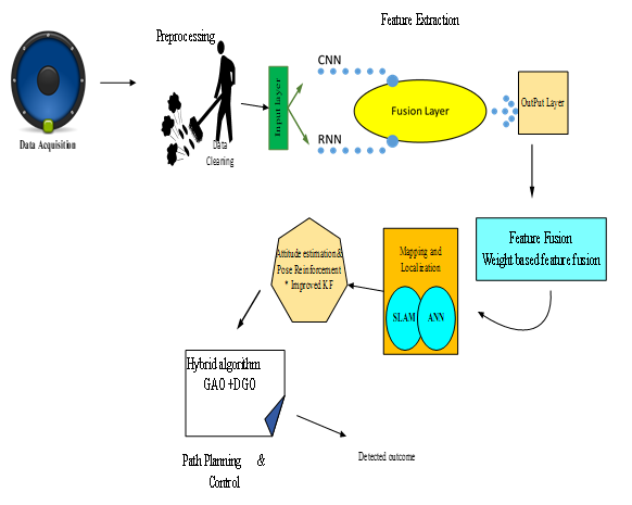
Figure 1: Over all flow diagram of the model

Preprocessing

In this proposed methodology, the preprocessing stage collects the data from sensors by including lidar, cameras, IMU, and potentially other advanced sensors like cameras or RGB-D sensors.

Sensors

A sensor is a device that perceives alterations to its surroundings and reacts to an output from another system.

Lidar

Robots can traverse their surroundings with the help of LiDAR (light detection and ranging) technology, which offers object perception, object recognition, and collision avoidance. Real-time information on the robot’s surroundings, including walls, doors, people, and various other objects, is provided via LiDAR sensors.

Cameras in Robot navigation

Cameras are incredible tools that contain two sensors in one. A camera first precisely calculates the direction of points in space. Second, computer vision algorithms can examine the 2D images captured by the sensor in order to identify things and assess the environment in front of the robot.

IMU

A group of sensors are the foundation of an IMU, an electronic device that uses the data produced by the sensors. Gyroscopes, accelerometers, and even magnetometers are examples of these basic sensors. Depending on the type of IMU, the information produced relates to three different aspects: acceleration, angular velocity, and orientation.

Depth Cameras or RGB ID sensors

With the use of depth-sensing cameras, machines can now comprehend their surroundings in three dimensions. In applications like vision-guided robots, inspection, and monitoring, depth cameras have grown in importance due to the deeper information they provide. A specific kind of depth camera known as an RGBD camera outputs both depth (D) and color (RGB) data in real-time.

Feature Extraction

In this research, from the preprocessing sensor data features are extracted by the use of deep neural networks like Convolutional Neural Networks and Recurrent Neural Networks.

Convolutional Neural Network

Convolutional layers (Conv), pooling layers (Pool), and fully connected layers (FC) are depicted in Figure 1 using the naming pattern of current common convolutional neural networks. Four convolutional layers, three pooling layers, and two fully linked layers make up the proposed network. To improve the local contrast, each convolutional layer is connected with a max-pooling layer. Analyse camera pictures using a CNN. When removing spatial characteristics from images, CNNs work effectively. After a number of convolutional layers, pooling layers will be used to create the CNN. Hierarchical characteristics from images are learned by these levels.

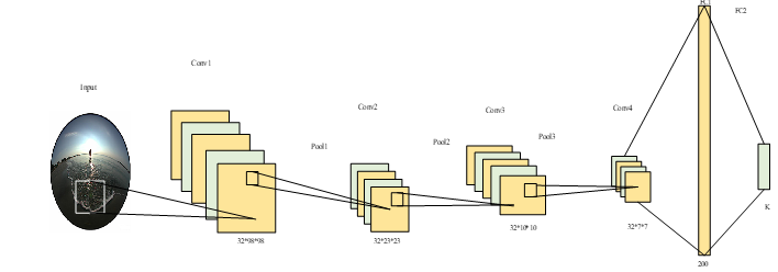
Figure 2: CNN Framework

A Convolutional Neural Network is an advanced deep-learning algorithm specialized in processing images. It adeptly identifies and distinguishes features and objects within images through learnable weights and biases. Unlike traditional methods that require manual filter engineering, ConvNet autonomously learns these filters and attributes. This reduces preprocessing efforts. The fundamental components of a ConvNet include the convolution layer (a), which extracts features; the pooling layer (b), which down samples data; the activation function (c), which introduces nonlinearity; and the fully connected layer (d), which performs the final classification. These elements collectively enhance the network’s capacity to recognize intricate patterns and objects in images. Figure 2 illustrates the CNN framework.

Convolutional layer

A convolutional neural network’s basic layer, the convolution layer, is located at its center. The response of related inputs within its receptive field is defined by this crucial layer. By applying kernels to the height and width of the input data, the layer convolutions generate a 2-D activation map by calculating the dot product between the input and filter values. Through this procedure, the CNN quickly learns about filters that turn on when certain features are detected at specified spatial regions in the input. The network’s aptitude for image and pattern recognition tasks depends on its innate capacity to identify as well as localize elements.

Pooling layer

Subsampling layers are essential for integrating local or global features in the CNN architecture. Reduced spatial dimensions are achieved by incorporating individual neurons’ outputs from one layer into those of the following layer. These reductions in size limit computations and parameters, speeding up processing while avoiding overfitting. This pooling layer type, which is usually referred to as max pooling, is recognised for its efficiency. Subsampling layers improve the network’s speed and efficiency by aggregating data and retaining key characteristics, making it better able to spot intricate patterns in a variety of data.

Fully connected layer

Similar to the traditional multi-layer perceptron, fully connected layers are essential components of deep neural networks. For classification or regression problems, they produce predictions using activations. Through matrix multiplication and bias addition, every activation from the preceding layer is linked to this one, enabling thorough information sharing and prediction creation.

RNN

Use an RNN to detect temporal connections and sequences in sensor data. For sequential data, Long Short-Term Memory (LSTM) is an appropriate choice. Figure 3 illustrates the schematic diagram of the circulating neural network, and C is the neural network unit, also known as the cyclic neural network unit. The input and output of are xt and ht, respectively. The RNN’s hidden layer is connected to both the previously encountered input features as well as the current input. The parameters of the network are updated via traversing time backpropagation, and it only requires one set of the neural network structure C. Ordinary RNNs struggle to handle long-distance dependence due to gradient expansion and gradient disappearance issues. Numerous derivative networks exist for recurrent neural networks (RNNs).

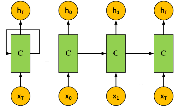
Figure 3: RNN

A popular network is the long short-term memory (LSTM) network. The fully connected (FC) hidden layer of a standard RNN is swapped out for units in LSTM. Figure 4 displays its schematic diagram.

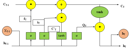
Figure 4: LSTM

Due to its ability to handle long-term dependencies, LSTM has solved the issue with conventional RNNs. Gate ft, which is constructed by three Sigmoid functions, is forgotten when Ct inputs gate it. The memory for previous status information is managed by the output gate to. Additionally, the gated recurrent unit (GRU), which combines the input gate and forgetting gate, is a superior variant structure of the LSTM.

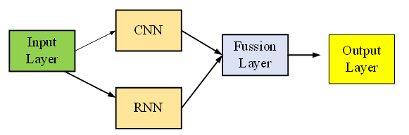
Figure 5: Feature Extraction flow

Figure 5 shown in Above, The technique makes use of neural networks, notably convolutional neural networks (CNNs) for processing camera pictures, to extract features from sensor data via deep learning. Through a stack of convolutional and pooling layers, CNNs are excellent at capturing spatial characteristics inside images, enabling the hierarchical learning of visual attributes. Recurrent neural networks (RNNs), such as the Long Short-Term Memory (LSTM) network, are used to take into account temporal correlations within sensor data sequences. These RNNs can handle sequential data with ease. An input layer, a CNN layer for image data, and an RNN layer for sequential data make up the processing pipeline. The outputs of the RNN and the CNN-based representations of the camera and lidar data are combined in a separate fusion layer. The final output layer achieves the desired outcomes and offers a comprehensive method of feature extraction and representation for thorough sensor data analysis.

Feature Fusion

After extracting the features, perform feature fusion using a weight-based approach by computing the weighted sum of features. This method involves multiplying each feature by its designated weight and then aggregating them into a single combined feature, resulting in a customized and effective representation. Weighted-based feature fusion plays a crucial role in enhancing robot navigation in complex and dynamic environments. In the context of robotics, it involves amalgamating data from various sensors and feature sources with different degrees of importance. By assigning appropriate weights to these sources, robots can make more informed decisions and navigate efficiently. For instance, a robot equipped with cameras, LIDAR, and ultrasonic sensors can benefit from weighted-based feature fusion. In a cluttered indoor environment, LIDAR data might be highly valuable for obstacle detection and avoidance. Therefore, it could be assigned a higher weight in the fusion process. Meanwhile, the camera data could be leveraged for recognizing landmarks or reading signage, contributing to localization and path planning but with a lower weight due to potential occlusions and lighting variations. Ultrasonic sensors, sensitive to immediate obstacles, could receive a moderate weight.

By skillfully combining these sensor inputs through weighted fusion, the robot can adapt its navigation strategy based on the context, focusing on critical information while filtering out less relevant data. This approach enables robots to make real-time decisions that balance safety and efficiency, ultimately leading to smoother and more reliable navigation in diverse and challenging environments, from warehouses to hospitals and beyond. Weighted-based feature fusion is an indispensable tool for ushering in the next era of autonomous robotics.

The general equation for weighted-based fusion can be represented as follows:

F=(ω1*m1)+(ω2*m2)+…..(ωn*mn) (1)

Where F is the resulting fused value, which combines information from multiple measurements or features. ω1,ω2….ωn are theweights assigned to each measurement or feature. These weights can be fixed or learned. m1,m2,…mn are the individual sensor measurements or feature values.

The choice of weights and how they are determined (fixed or learned) depends on the specific robot navigation task and the characteristics of the sensors or features involved. These weights are designed to give more importance to reliable or informative measurements while downplaying less reliable ones. The fused value can then be used in navigation algorithms to make decisions about the robot’s movement and actions based on the combined sensor information.

Mapping and Lozalization

SLAM Algorithm with Deep Learning Integration

SLAM uses the robot’s location to create an environmental map, which is then used to calculate the robot’s position using the previously created map. They support one another. It can be summarised as using sensor data to address the issues of creating an environmental map and detecting its own orientation at the same time. In accordance to the mobile robot’s motion model, process noise and control input cause the robot’s posture to alter over time. The robot’s motion model can be stated as

X_T=H(X_T-1,U_T)+δ_T (2)

The robot’s state vector X_T, which includes different factors including location, heading angle, and speed, describes the robot in its current state of posture, which is usually nonlinear, H is a state transition model. U_T , is the control input data, and δ_T it represents the time-independent random noise in the process of robot movement, with a mean value of 0, and a covariance of q_T.

The robot on the move enters an unknown environment from an unknown position, moves while using its own sensors to gather environmental data, uses this data to continuously create and update the environmental map, and at the same time chooses its position and posture based on the sensor data and the created environmental map. It is possible to sum up the localization and mapping of SLAM as a process of “estimation”-“observation”-“correction.” Figure 6 displays the diagram of the system state.

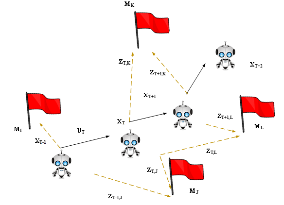
Figure 6: System State Diagram

X_T Displays the mobile robot’s current state, M_Jthe environment’s attributes, U_T the robot’s control input, and the sensor’s observed measurement. The system state at a given time, the input at that time, and Z_T the observed sensor measurement at that time are all tied to the current state of the robot. It is required to correct the position because the sensor will have some mistakes by monitoring external environmental landmarks, calculating the robot’s pose based on the observed landmarks, and then estimating the robot’s initial estimated stance using the landmarks’ calculated pose. The estimating inaccuracy decreases with the number of environmental features observed.

In order to estimate a robot’s position and pose as well as the location of surrounding landmarks, SLAM relies heavily on assessing sensors’ perception of the surrounding environment. Currently, lidar, camera, sonar sensor, and other sensors are the most common ones used in SLAM to sense environmental data.

Artificial Neural Network

The following D2D communication example is retained to illustrate ANN power control. It is a separate application: the supplied manuscript does not establish how its channel gains and power outputs map to robotic localization.

Artificial neural networks are configurations that are frequently employed in machine learning. Neurons are the building blocks of a neural network, which is divided up into layers. Each layer may have one or more neurons, and depending on where it is in the neural network, it may be an input layer, hidden layer, or output layer. The first and last layers are referred to as the input layer and output layer, respectively. There are several layers, each of which is referred to as a hidden layer, in between the input and output layers.

The optimization problem in equation is based on the mathematical relationship between the cellular channel gains and the D2D channel gains. The relationship between cellular and D2D channel gains in mobile networks is unknown, and it cannot even be inferred analytically from any known properties of mobile networks and recommended using an artificial neural network to automatically learn this relationship and modify the D2D pairs’ transmission strength accordingly (ANN). To put it more precisely, the ANN can be compared to a regulator that controls the D2D pair’s transmission power solely based on the data about cellular channel gains that D2D users transmit to base stations. The aim of the optimization in Eqn. (3) for the binary power control is to set the transmission power of each D2D pair to either ork_m =k_minor k_m=k_max . Setting the transmission power for N D2D pairs is the challenge associated with identical binary classification. We suggest the use of a fully connected ANN to create a mapping between cellular channel gains and the best binary transmission power setting for each m^th D2D pair that maximises the total capacity of D2D pairs.

Figure 7 displays the ANN for binary classification. The proposed ANN is made up of an input layer C=(C₁, C₂,……,C_m), hidden layers S=(S₁,S₂….S_m), and an output layer B=(B₁, B₂,….B_m). The cellular channel gains from the D2D users to the base stations are aligned by the input layer of the suggested ANN, which has an input layer with an input vector. The term,Out_c0 =K_1,1 , K_1,2,………..K_X,W produced by the input layer, has a length of X×Wand is a vector that represents the cellular channel gains between base stations and D2D users.

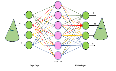
Figure 7: ANN Architecture

Because the sigmoid function’s value falls between 0 and 1, the output of the ANN will be, which shows the likelihood that. The transmission power for the m^th D2D pair is therefore set to:

k_m={k_max if out_B >0.5 ; k_{min( )} otherwise (3)

An activation function Φ is used to describe a basic model of a neuron by applying it to a linear combination of input data C==(C₁, C₂,……,C_m), weights D=D₁,D₂,….D_w, and bias constant y. Consequently, the output B is such that B=Φ(U) and where U=y+∑_r=1^w(D_rC_r). This output is then transmitted to the following layer as input data along with all of its other outputs, continuing the process until the output layer produces the final output.

Since the activation function Φ of the most popular neuron model, the sigmoid neuron, is the sigmoid function Φ(U)= (1)/(1+e^–ηU) , the output is calculated as follows.

B=(1)/(1+e^{-η∑_r=1w(D_rC_r-y)}) (4)

Since gradient descent is a common method for adjusting the weights and bias, the sigmoid neuron’s popularity can be attributed to how simple it is to obtain the partial derivative of this function. The backpropagation and feed-forward processes make these adjustments.

The transmission power of the D2D pairs cannot be calculated using a straightforward mathematical relationship between the cumulative capacity of the D2D pairs and the cellular channel gains. Therefore, in order to maximise the sum capacity of D2D pairs, we offer an offline supervised learning-based technique in which the ideal binary transmission powers are discovered following a thorough search. The suggested artificial neural network is then given the transmission power of the m^th D2D pair as a targeted class linked to a set of cellular channel gains as features.

Attitude Estimation &Pose reinforcement

A thorough introduction to the visual inertial navigation system’s attitude fusion estimation algorithm based on KF will be provided. Figure 8,9 s depicts the algorithm flow chart.

It is important to identify the state equation that agrees with the linear system, i.e., to linearize KF, in order to process the KF more intuitively. Although it is standard practice, using error state quantity to express system modeling can reduce data redundancy and increase operational efficiency. Instead of using the arithmetic error between rotation and rotation estimation, error quaternion is employed to define the error quantity. The tiny rotation between an estimated amount and the real state quantity is represented by the error quaternion two in this case, and this error is defined by multiplication, as illustrated in the following formula:

δQ̂=Q⨂Q̂^-1 (5)

Given that the second error quaternion is a very small rotation, it can be written as an approximately small angle error. A small angle error is defined as follows.

δQ=[[δQ] ; [δQ_W]]=[[K̂sin⁡((δθ)/(2))] ; [cos⁡((δθ)/(2))]]=[[(1)/(2)δθ] ; [1]] (6)

Where δQ and δQ_W are the actual and imaginary components of a microrotation, respectively. Currently, the error state quantity δXcan be stated using the formula below, where ∆B is the mistake:

δX=[[δθ] ; [∆B]] (7)

The inertial navigation system’s state equation can be effectively approximated using the error state equation. The high-frequency output of the IMU for attitude estimation tends to accumulate substantial errors over time. To enhance system robustness, integrating the low-frequency output from visual SLAM as the IMU’s attitude output proves beneficial. The visual attitude estimation Q_C^Wnot only signifies the transformation from camera to world coordinates but also serves as a crucial observation value Z within the filtering process. This integration enhances overall performance and accuracy. The joint observation matrix’s expression for the available observation equation is as follows:

h=[0_3×3 i_3×3 (8)

From then, the observation matrix and observation noise variance matrix may be used to determine the updating process of KF, and the precise stages are shown in the following formula:

k_K=p_K|K-1 h_K^t(h_Kp_K|K-1 h_K^t+r_K)^-1 (9)

X̂_K=X̂_K|K-1+k_K(Z_K-h_KX̂_K|K-1) (10)

p_K=(i-k_Kh_K)p_K|K-1 (11)

A vector that specifies a feature’s location and other characteristics mathematically represents the feature. The environmental features that sensors measure is often referred to as point features. The environment’s I th characteristic can be stated by P_I, which is referred to as

P_I=[[X_I] ; [Y_I]] (12)

When the status of a feature changes infrequently from time K to the time K+1, it can be considered static, as showed by the following examples:

P_I(K+1)=P_I(K)=P_I (13)

Enhance attitude estimation by merging traditional Kalman filtering and optimized neural networks. These fusion augments pose accuracy for improved results in attitude estimation, delivering superior performance.

Path Planning and Control

To develop a reinforcement learning-based control policy that takes the SLAM-derived map and current pose as input to generate robot control commands for navigation and to use hybrid optimization algorithms that combine traditional optimization methods with reinforcement learning to plan optimal collision-free paths in dynamic environments.

Green Anaconda Optimization

The green anaconda (Eunectes murinus), a species of boa found in South America, is sometimes referred to as the big anaconda or common aquatic boa. It is one of the most lengthy and largest non-venomous constrictor snakes in the world. It resembles other boa species. There have been claims that green anacondas may grow to a length of 5.21 m. The average length of the female species is 4.6 meters, whereas the average length of the male species is 3 meters. According to reports, green anacondas can weigh anywhere from 30 to 70 kg. The bodies of green anacondas are olive green and covered with black spots. They have a thinner head compared to their body size, which is differentiated by orange-yellow striping. With its eyes on its head, the green anaconda can swim through the water and emerge from it without revealing its body. Green anacondas may swallow prey bigger than their own heads due to their flexible jaw bones.

Green anacondas seek animals to supplement their diversified diet. Fish, birds, reptiles like tortoises and animals like agoutis are all part of this diet. Additionally, there are claims that green anacondas occasionally pursue prey species weighing more than 40 kg for their food. The majority of the time green anacondas spend in or near water. Although they move slowly on land, they can swim quite quickly and are very nimble in the water. The green anaconda hunts by concealing itself below the water’s surface and protruding its snouts above the surface. It is a fierce hunter that strikes, wraps itself tightly around its prey, and suffocates it before devouring it whole. Males start looking for females as mating season comes. Males rely on pheromones left by females to confidently locate and approach them. Males repeatedly flick their tongues throughout this procedure in order to detect molecules that signal the females. The green anaconda exhibits prominent mating behaviors during the breeding period, including pursuing females and adjusting its hunting approach. GAO technique effectively captures the cognitive processes involved its natural behaviors through mathematical modeling. The Green anacondas represent the members of the proposed GOA, which is a population-based metaheuristic algorithm. Each green anaconda in the search space represents a potential solution for the issue. Each green anaconda can be represented as a vector, and the populations can be represented as a matrix.

X=[X₁ ; ⋮ ; X_i ; ⋮ ; X_N]=[x_1,1… x_1,d… x_1,m ; ⋮ ⋱ ⋮ ⋱ ⋮ ; x_i,1… x_i,d… x_i,m ; ⋮ ⋱ ⋮ ⋱ ⋮ ; x_N,1… x_N,d… x_N,m] (14)

Before running the algorithm, the starting location of each green anaconda within the search space is randomly generated.x_i,d=lb_d+r_i,d∙(ub_d-lb_d), i=1,2,……,N and d=1,2,…..,m

where X is a matrix of population of GAO, Xi denotes the green anaconda in the i^th position, x_i,d denotes the d^th dimension of search area, N denotes total count of green anacondas, amount of decision variables is denoted by m, r_i,d are randomly chosen numbers from 0 to 1, and lb_d, ub_d denotes the lower and upper limit of the d^th decision variable. Use recommended values to assess the objective function. According to the equation below, a vector may be used to mathematically describe this collection of determined values for the goal function.

F=[F₁ ; ⋮ ; F_i ; ⋮ ; F_N]=[F_(X1) ; ⋮ ; F_(Xi) ; ⋮ ; F_(XN)] (15)

In Eq. (15) Where, F is the estimated target function’s vector, F_i is the target function that was computed using the i^th green anaconda. The green anaconda positions are updated each iteration, with the best candidate solution chosen by comparing objective function values.

Mathematical representation

Phase 1: Breeding period (Exploration)

The female species emit pheromones for male species to identify during breeding period. This tactic causes significant shifts in their places, showcasing the GAO’s exploratory capabilities in precise problem-solving and worldwide search. The design assumes that female species with better objective function values are considered for each of them,

CFLⁱ={X_ki : F_ki<F_i and k_i≠i} (16)

In Eq. (16) Where, i = 1,2,…..,N and k_i∈{1,2,…,N} Here CFLⁱ is the set of location of females in the i^th big anaconda and the value k_i represents the location in the objective function vector of the component with the highest objective function value and row number in the GAO population matrix.

The equation that is used to determine the likelihood of pheromone concentration for each species of matter that a GAO member represents.

PC_jⁱ=(CFF_jⁱ-CFF_maxⁱ)/(∑_n=1ⁿⁱ(CFF_nⁱ-CFF_maxⁱ)) , i=1,2,….,N and j=1,2,…..,n_i (17)

Here, PC_jⁱ is the i^th green anaconda’s j^th female’s pheromone concentration probability, CFFⁱ is the vector representing the set of objective functions of the i^th big anaconda candidate female, CFF_jⁱ is its j^th value, CFF_maxⁱ is its maximum value, and ni is the number of candidate females. The GAO design assumes a big anaconda randomly selects a material. The candidate girls’ cumulative probability is calculated,

C_jⁱ=PC_jⁱ+C_j-γⁱ , where i=1,2,…..,N, j=1,2,…..,m and C₀ⁱ=0 (18)

and the selected species is determined using the equation,

SFⁱ=CFL_jⁱ : CFL_j-1ⁱ<r_i,j<C_jⁱ (19)

where SFⁱ is the chosen female for the i^th big anaconda, C_jⁱ is the function of cumulative probability of j^th female, and A random number named r has a normal distribution and a range of 0 to 1. Eq. (20) is used to determine a random position for the chosen female species. If the objective function value improves, the green anaconda’s position is updated.

x_i,d^P1=x_i,d+r_i,d∙(SF_dⁱ-I_i,d∙x_i,d), i=1,2,….,N and d=1,2,……, m. (20)

X_i={X_i^P1 , F_i^P1<F_i ; X_i , else (21)

Where, x_i,d^P1 is the d^th dimension, F_i^P1 is the function value of the target, r_i,d are randomly chosen numbers from 0 to 1. SF_dⁱ denotes the i^th green anaconda’s chosen female’s d^th dimension. I_i,d are random numbers from the set {1,2}, 𝑁 is the total count of big anacondas, and 𝑚 gives the count of decision variables.

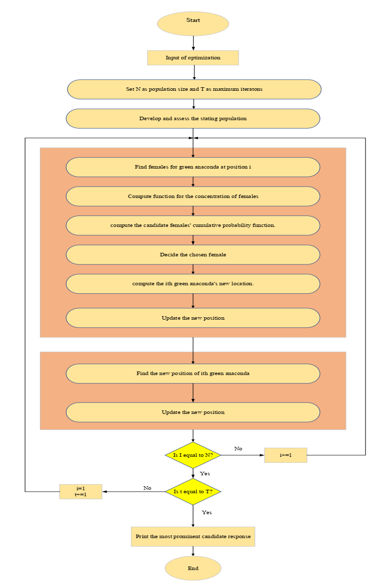
Figure 8: Flowchart of GAO

Phase 2: Hunting tactics (Exploitation)

Big anacondas are underwater predators that ambush and wait for prey. They attack, surround, suffocate, and swallow prey. In the second phase of GAO, population members’ positions are updated based on their hunting strategy. This exploitation allows for better solutions near discovered solutions. To simulate this, random positions are generated near each anaconda, and if the objective function value improves, the location is updated.

Random position is generated using the equation,

x_i,d^P2=x_i,d+(1-2_ri,d)(ub_d-lb_d)/(t), i=1,2,…..,N, d=1,2,……,m, and t=1,2,….,T (22)

Position is updated as,

X_i={X_i^P2 , F_i^P2<F_i ; X_i , else (23)

where X_i^P2 denotes the second phase’s updated position for the i^th green anaconda, x_i,d^P2 is its 𝑑th dimension, F_i^P2 is its target function value, 𝑡 gives the count of iteration, and 𝑇 is the maximum number of algorithm iterations.

Darts game optimizer

Anyone may enjoy the sport of darts, regardless of age or gender. Despite the apparent simplicity of the game, the players’ talent has a significant impact on the point total. This game may seem simple but the players should be skilled in points collection. This game includes properties like dartboards and darts. Each throw is scored by allocating 50 and 25 points to the inner and outer bulls, respectively. Each sector’s score is shown above it. The score is quadrupled if the darts land in the inner narrow ring and doubled if they land in the outer narrow ring. The fact that the dartboard’s Centre is the fifth-highest scoring location in the game is significant. The potential of the darts game is used to create and launch a novel optimizer in the darts game optimizer. Players in this game are searcher agents from DGO, and their objective is to achieve the highest possible.

Mathematical model

A matrix is used to represent the population of players, with each row denoting a single individual and each column denoting that player’s many traits. This matrix’s number of columns really corresponds to the number of issue variables and the recommended values for those variables.

X=[X₁ ; ⋮ ; X_i ; ⋮ ; X_N|x₁¹…x₁^d…x₁^m ; ⋮ ⋱ ⋮ ⋱ ⋮ ; x_i¹…x_i^d…x_i^m ; ⋮ ⋱ ⋮ ⋱ ⋮ ; x_N¹… x_N^d… x_N^m ] (24)

Here, m is the total count of variables, N is the number of players, X is the matrix of players, and x_i^d is the ith participant’s d-th dimension. Useful data is collected by putting Xi in the function of fitness and is displayed in the following equations,

F_b=min⁡(fit)_N×1 (25)

X_b=X(location ofmin((fit)), 1∶m)

F_w=max(fit)_N×1 (26)

X_w=X(location ofmax((fit)), 1∶m)

Fⁿ=(fit-F_w)/(∑_j=1^N((fit_j-F_w))) (27)

P_i=(F_iⁿ)/(max⁡(Fⁿ)) (28)

Here, the best and worst fitness values are denoted using F_b and F_w respectively. Simultaneously, best and worst variables are given as X_b and X_w. Fⁿ is the normalize fitness function and P_i gives the probability of i^th participant.

Dartboard includes 82 distinct scoring zones. In each round, each player may throw three darts. There are two things that affect where the darts land on the dartboard: player luck and ability. On the dartboard, there are six distinct sorts of sectors with various areas.

Table 1: Specification of dartboard sectors

The above table 1 gives the angle and areas for each sector of the dartboard. The inner diameter of double and triple ring is 8 mm. The inner diameter of inside bull is 12.7 mm and outside bull is 31.8 mm. From the center bull, the outside edge of bull is 107 mm. The overall dartboard diameter is 451 mm. Consequently, each player’s throwing score is modelled and computed in the below equations,

C_i=round(82×(1-P_i)) (29)

SC_i={S(1∶C), rand<P_i ; S(C+1∶82), else (30)

s_i=SC_i(k)&1≤k≤82 (31)

s_iⁿ=(∑_throw=1³(s_i^throws))/(180) (32)

Where, SC_i is the score of players i, S is the matrix of scores from high to low, s_i denotes the point scored by player i at each throw, and the normalised score of players i is s_iⁿ. Last but not least, the values of the issue variables are changed using the new status of each participant.

X_i=X_i+rand(1,m)×(X_b-3s_iⁿX_i) (33)

The proposed DGO algorithm can solve optimization problems with 50 players and 1000 repetitions as a stop condition. Each player represents an m-member vector representing a suggested answer to the problem, with the variables evaluated by placing them in the objective function.

The steps in darts game optimization algorithm are picturized below. This optimization algorithm is easily understandable and implemented. It can be used on many optimization problems like, single-objective and multi-objective optimization, as well as continuous and discrete optimization tasks. Unlike traditional optimization algorithms that rely on populations of solutions, Darts Game Optimization operates with a single solution, simplifying the algorithm’s management and control. In summary, the Darts Game Optimization Algorithm offers simplicity, versatility, global search capabilities, and other advantages that make it a promising approach for solving a wide range of optimization problems efficiently and effectively.

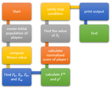
Figure 9: Steps in DGO algorithm

Result And Discussion

The framework combines sensor fusion, deep learning, SLAM and reinforcement learning. The classification statistics below are reproduced as reported, but no common confusion matrix, labeled task definition or navigation benchmark is supplied. Sensitivity and recall differ, and the reported false-positive and false-negative rates do not complement specificity and sensitivity. These values cannot establish trajectory accuracy, collision avoidance or superiority in deployed robot navigation. The D2D power-control example in the ANN section illustrates a separate application; its mapping to robot localization is not specified.

Experimental Setup

In this research, the proposed model is implemented in MATLAB to get the best accuracy, with the metrics like sensitivity, specificity, accuracy, Precision, F1-Score, recall, FNR, FPR, NPV, MCC.

Overall performance of the proposed model

Table 3 reports sensitivity 0.999, specificity 0.987, accuracy 0.99, precision 0.996, recall 0.9707, F-measure 0.964, NPV 0.985, FPR 0.005, FNR 0.028 and MCC 0.931 for RL-DLT-SLAM. These are the manuscript’s reported values. The comparison includes CNN, RNN, LSTM, GRU and DNN models, but the metric inconsistencies and unspecified evaluation task prevent a verified claim of overall superiority. NPV means negative predictive value, rather than false-predictive value.

Table 3: Overall performance of the proposed model

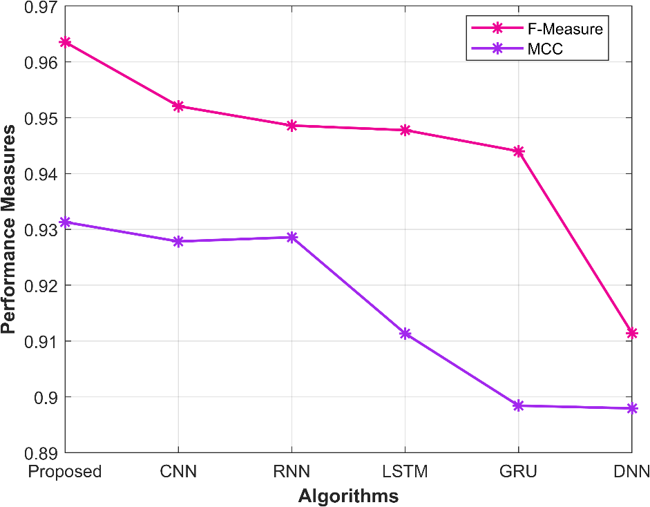
Figure 10: Graphical representation of the performance metrics F-Measure and MCC of the proposed model

The above figure 10 illustrates the graphical format of the performance metrics F-Measure and MCC of the proposed model with another comparative model. From this graphical representation it is clear that the F-Measure and MCC value of the proposed model is higher than the other comparative models like CNN, RNN, LSTM, GRU, DNN.

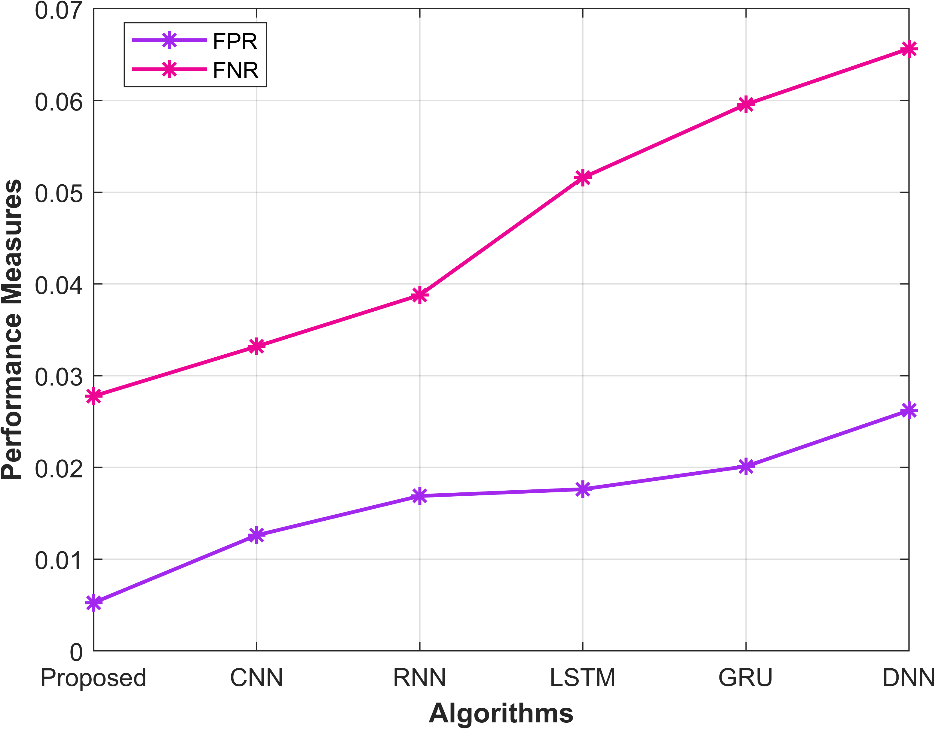
Figure 11: Graphical representation of the performance metrics FPR and FNR of the proposed model

The above Figure 11 illustrates the graphical format of the performance metrics FPR and FNR of the proposed model with another comparative model. From this graphical representation it is clear that the FPR and FNR value of the proposed model is lower than the other comparative models like CNN, RNN, LSTM, GRU, DNN.

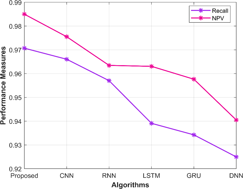
Figure 12: Graphical representation of the performance metrics Recall and NPV of the proposed model

The above Figure 12 illustrates the graphical format of the performance metrics Recall and NPV of the proposed model with other comparative model. From this graphical representation it is clear that the Recall and NPV value of the proposed model is higher than the other comparative models like CNN, RNN, LSTM, GRU, DNN.

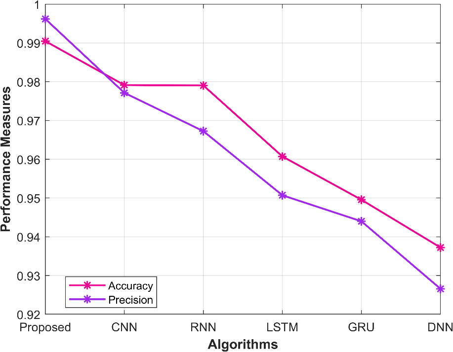
Figure 13: Graphical representation of the performance metrics Accuracy and precision of the proposed model

The above Figure 13 illustrates the graphical format of the performance metrics accuracy and precision of the proposed model with another comparative model. From this graphical representation it is clear that the Accuracy and precision value of the proposed model is higher than the other comparative models like CNN, RNN, LSTM, GRU, DNN.

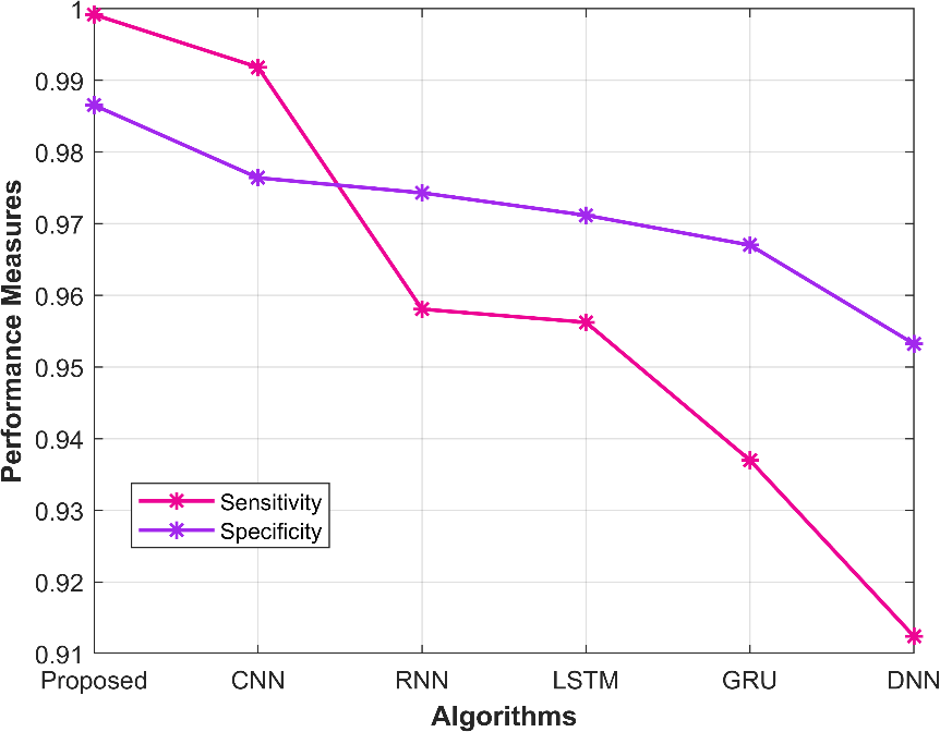
Figure 14: Graphical representation of the performance metrics Sensitivity and Specificity of the proposed model

The above Figure 14 illustrates the graphical format of the performance metrics Sensitivity and Specificity of the proposed model with another comparative model. From this graphical representation it is clear that the Sensitivity and specificity value of the proposed model is higher than the other comparative models like CNN, RNN, LSTM, GRU, DNN.

Conclusion

In conclusion, our proposed methodology represents a holistic and cutting-edge approach to autonomous robotics. We start by meticulously gathering data from a diverse array of sensors, ensuring a rich and comprehensive understanding of the robot’s environment. This data is then subjected to a sophisticated feature extraction process, employing Convolutional Neural Networks (CNNs) for spatial analysis and Recurrent Neural Networks (RNNs), specifically Long Short-Term Memory (LSTM) networks, for temporal context capture. The integration of these features is accomplished through weight-based fusion, allowing us to harmonize information from different sensors effectively. We then elevate the capabilities of our robots through the implementation of Deep Learning-SLAM, enhancing mapping and localization with optimized neural networks. Furthermore, the fusion of Kalman filtering and neural networks significantly refines attitude estimation and pose accuracy. Our path planning and control strategy introduce reinforcement learning-based policies that leverage SLAM-derived maps and real-time pose data for precise and adaptable navigation. Finally, we employ hybrid optimization algorithms that bridge traditional optimization methods with reinforcement learning, enabling the robot to autonomously plan collision-free paths in dynamic and complex environments. This comprehensive methodology equips our autonomous robots with the intelligence and adaptability required to navigate, perceive, and interact with their surroundings, ushering in a new era of advanced and versatile robotic systems.

References

[1] Qiu, X., Feng, Z., Xu, T., Yang, X., & Zhang, X. (2021). Research on intention flexible mapping algorithm for elderly escort robot. Sciesntific Programming, 2021(8), 1-14.

[2] Tian, Y., Yang, W. H., & Huang, X. Y.. (2021). A visual navigation algorithm for landing based on 3d model of small body. SCIENTIA SINICA Physica, Mechanica & Astronomica, 52(1), 214503.

[3] Guo, X. D., Wang, Z. B., Zhu, W., He, G., Deng, H. B., & Lv, C. X., et al. (2022). Research on dso vision positioning technology based on binocular stereo panoramic vision system. Defence Technology, 18(4), 593-603.

[4] Li, Q., Kang, J., & Cao, X. (2021). Research on slam based on rbpf algorithm in indoor environment. Journal of Physics: Conference Series, 1971(1), 012066 (6pp).

[5] M Serveries, Renaudin, V., Dupuis, A., & Antigny, N. (2021). Visual and visual-inertial slam: state of the art, classification, and experimental benchmarking. Journal of Sensors, 2021(1), 1-26.

[6] Ma, T. , Bai, N. , Shi, W. , Wu, X. , & Zhao, C. . (2021). Research on the application of visual slam in embedded gpu. Wireless Communications and Mobile Computing, 2021(6), 1-17.

[7] Shen, K., Qiu, Q., Wu, Q., Lin, Z., & Wu, Y. (2021). Research on the development status of agv parking robot based on patent analysis. Journal of Physics Conference Series, 1905(1), 012018.

[8] Alkendi, Y., Seneviratne, L., & Zweiri, Y. (2021). State of the art in vision-based localization techniques for autonomous navigation systems. IEEE Access, PP (99), 1-1.

[9] Magallanes, E. O., Aldana-Murillo, N. G., Avina-Cervantes, J. G., Ruiz-Pinales, J., & Ledesma, S. (2021). Transfer learning for humanoid robot appearance-based localization in a visual map. IEEE Access, 9(99), 6868-6877.

[10] Gao, Y., Zheng, X., Mao, X., Tian, H., & Sun, S. (2021). Research on moon surface positioning and navigation method based on stellar vector measurement. Journal of Physics Conference Series, 1786(1), 012036.

[11] Ma, G., & Pan, X. (2021). Research on a visual comfort model based on individual preference in china through machine learning algorithm. Sustainability, 13(14), 7602.

[12] Shi, L., Ding, X., Li, M., & Liu, Y. (2021). Research on the capability maturity evaluation of intelligent manufacturing based on firefly algorithm, sparrow search algorithm, and bp neural network. Complexity, 2021(3), 1-26.

[13] Wang, Z., Zhang, Q., Jia, T., & Zhang, S. (2021). Research on control algorithm of an automatic driving robot based on improved model predictive control. Journal of Physics: Conference Series, 1920(1), 012116 (6pp).

[14] Ye, J., & Xu, W. (2021). Research on machine learning algorithm based on contour matching modal matrix. Journal of Physics: Conference Series, 1883(1), 012006 (11pp).

[15] Zhang, X., Zhang, S., & Huai, S. (2021). Low-power indoor positioning algorithm based on ibeacon network. Complexity, 2021(1), 1-10.

[16] Jin, Q., Tang, C., & Cai, W. (2021). Research on dynamic path planning based on the fusion algorithm of improved ant colony optimization and dynamic window method. IEEE Access, PP (99), 1-1.

[17] Fang, B., Mei, G., Yuan, X., Wang, L., & Wang, J. (2021). Visual slam for robot navigation in healthcare facility. Pattern Recognition, 113(12), 107822.

[18] Tolani, V., Bansal, S., Faust, A., & Tomlin, C. (2021). Visual navigation among humans with optimal control as a supervisor. IEEE Robotics and Automation Letters, PP(99), 1-1.

[19] Morad, S. D., Mecca, R., Poudel, R., Liwicki, S., & Cipolla, R… (2021). Embodied visual navigation with automatic curriculum learning in real environments. IEEE Robotics and Automation Letters, PP(99), 1-1.

[20] Meng, X. , Xiang, Y. , & Fox, D. . (2021). Learning composable behavior embeddings for long-horizon visual navigation. IEEE Robotics and Automation Letters, PP(99), 1-1.

[21] Leonard, J.J. and Bahr, A., 2016. Autonomous underwater vehicle navigation. Springer handbook of ocean engineering, pp.341-358.

[22] Yang, G., Chen, Z., Li, Y. and Su, Z., 2019. Rapid relocation method for mobile robot based on improved ORB-SLAM2 algorithm. Remote Sensing, 11(2), p.149.

[23] Lee, Y.H. and Medioni, G., 2016. RGB-D camera based wearable navigation system for the visually impaired. Computer vision and Image understanding, 149, pp.3-20.

[24] Heo, S. and Park, C.G., 2018. Consistent EKF-based visual-inertial odometry on matrix Lie group. IEEE Sensors Journal, 18(9), pp.3780-3788.

[25] Yang, T., Li, P., Zhang, H., Li, J. and Li, Z., 2018. Monocular vision SLAM-based UAV autonomous landing in emergencies and unknown environments. Electronics, 7(5), p.73.

[26] Schneider, T., Dymczyk, M., Fehr, M., Egger, K., Lynen, S., Gilitschenski, I. and Siegwart, R., 2018. maplab: An open framework for research in visual-inertial mapping and localization. IEEE Robotics and Automation Letters, 3(3), pp.1418-1425.

[27] Mutz, F., Veronese, L.P., Oliveira-Santos, T., De Aguiar, E., Cheein, F.A.A. and De Souza, A.F., 2016. Large-scale mapping in complex field scenarios using an autonomous car. Expert Systems with Applications, 46, pp.439-462.

[28] Pahlavan, K., Krishnamurthy, P. and Geng, Y., 2015. Localization challenges for the emergence of the smart world. IEEE Access, 3, pp.3058-3067…

[29] Brubaker, M.A., Geiger, A. and Urtasun, R., 2015. Map-based probabilistic visual self-localization. IEEE transactions on pattern analysis and machine intelligence, 38(4), pp.652-665.

[30] Li, B., Munoz, J.P., Rong, X., Chen, Q., Xiao, J., Tian, Y., Arditi, A. and Yousuf, M., 2018. Vision-based mobile indoor assistive navigation aid for blind people. IEEE transactions on mobile computing, 18(3), pp.702-714.

[31] McGuire, K.N., de Croon, G.C. and Tuyls, K., 2019. A comparative study of bug algorithms for robot navigation. Robotics and Autonomous Systems, 121, p.103261.

[32] Santoso, F., Garratt, M.A. and Anavatti, S.G., 2016. Visual–inertial navigation systems for aerial robotics: Sensor fusion and technology. IEEE Transactions on Automation Science and Engineering, 14(1), pp.260-275.

[33] Ranft, B. and Stiller, C., 2016. The role of machine vision for intelligent vehicles. IEEE Transactions on Intelligent vehicles, 1(1), pp.8-19.

[34] Zhang, X., Xian, B., Zhao, B. and Zhang, Y., 2015. Autonomous flight control of a nano quadrotor helicopter in a GPS-denied environment using on-board vision. IEEE Transactions on Industrial Electronics, 62(10), pp.6392-6403.

[35] Li, J., Qin, H., Wang, J. and Li, J., 2021. Openstreetmap-based autonomous navigation for the four wheel-legged robot via 3d-lidar and ccd camera. IEEE Transactions on Industrial Electronics, 69(3), pp.2708-2717.

[36] Kumar, G.A., Patil, A.K., Patil, R., Park, S.S. and Chai, Y.H., 2017. A LiDAR and IMU integrated indoor navigation system for UAVs and its application in real-time pipeline classification. Sensors, 17(6), p.1268.

[37] Chang, L., Shan, L., Jiang, C. and Dai, Y., 2021. Reinforcement based mobile robot path planning with improved dynamic window approach in unknown environment. Autonomous Robots, 45, pp.51-76.

[38] Rebecq, H., Horstschäfer, T., Gallego, G. and Scaramuzza, D., 2016. Evo: A geometric approach to event-based 6-dof parallel tracking and mapping in real time. IEEE Robotics and Automation Letters, 2(2), pp.593-600.

[39] Xu, H., Ding, Y., Li, P., Wang, R. and Li, Y., 2017. An RFID indoor positioning algorithm based on Bayesian probability and K-nearest neighbor. Sensors, 17(8), p.1806.

[40] Jiang, G., Yin, L., Jin, S., Tian, C., Ma, X. and Ou, Y., 2019. A simultaneous localization and mapping (SLAM) framework for 2.5 D map building based on low-cost LiDAR and vision fusion. Applied Sciences, 9(10), p.2105.

[41] Vivacqua, R.P.D., Bertozzi, M., Cerri, P., Martins, F.N. and Vassallo, R.F., 2017. Self-localization based on visual lane marking maps: An accurate low-cost approach for autonomous driving. IEEE Transactions on Intelligent Transportation Systems, 19(2), pp.582-597.

[42] Carreras, M., Hernández, J.D., Vidal, E., Palomeras, N., Ribas, D. and Ridao, P., 2018. Sparus II AUV—A hovering vehicle for seabed inspection. IEEE Journal of Oceanic Engineering, 43(2), pp.344-355.

[43] Li, H., Zhang, Q. and Zhao, D., 2019. Deep reinforcement learning-based automatic exploration for navigation in unknown environment. IEEE transactions on neural networks and learning systems, 31(6), pp.2064-2076.

[44] Thanpattranon, P., Ahamed, T. and Takigawa, T., 2016. Navigation of autonomous tractor for orchards and plantations using a laser range finder: Automatic control of trailer position with tractor. Biosystems Engineering, 147, pp.90-103.

[45] Ilci, V. and Toth, C., 2020. High-definition 3D map creation using GNSS/IMU/LiDAR sensor integration to support autonomous vehicle navigation. Sensors, 20(3), p.899.

Editorial Staff

Academic Master Education Team is a group of academic editors and subject specialists responsible for producing structured, research-backed essays across multiple disciplines. Each article is developed following Academic Master’s Editorial Policy and supported by credible academic references. The team ensures clarity, citation accuracy, and adherence to ethical academic writing standards

Content reviewed under Academic Master Editorial Policy.

• Editorial Staff

  Grid-Connected Solar PV Systems and Power Quality Review
• Editorial Staff

  Predicting Cardiovascular Diseases with PCA and Artificial Neural Networks
• Editorial Staff

  Maternal and Neonatal Outcomes Following Water Birth Systematic Review and Meta-Analysis
• Editorial Staff

  Electrospun Polymeric Nanofibers for Biomedical Applications