
Abstract
This study examines a Cascaded Fused Faster R-CNN research framework for lung cancer image classification. The workflow combines non-local means (NLM) and wavelet denoising, Cascaded SegNet segmentation, feature selection using LASSO and Elastic Net regularisation, and classification using a cascaded Faster R-CNN model. NLM uses similarities between image patches to reduce noise while preserving detail, and wavelet processing provides a complementary denoising stage. Cascaded SegNet extracts lung regions through successive processing stages. LASSO and Elastic Net are then used to identify informative features and reduce the feature-space dimensionality. The classification stage adapts a region-based object-detection architecture to the image-analysis task. The manuscript presents model-comparison tables and figures for the reported experiment. These results describe a computational research study and do not establish clinical diagnostic performance.
Keywords: Lung Cancer Prediction, Non-Local Means, Cascaded SegNet, cascaded fused Faster R-CNN.
Introduction
Worldwide, lung cancer accounts for a disproportionately high number of cancer-related deaths [1]. Improving patient outcomes and decreasing death rates from lung cancer requires early identification and an accurate prognosis of the disease [2]. With the developments in medical imaging technology and machine learning methods, computer-aided diagnostic systems have emerged as strong devices to help radiologists in the identification and prediction of lung cancer [3]. The prediction of lung cancer is only one area where deep learning-based algorithms have demonstrated substantial progress in recent years [4]. In order to extract features and classify lung cancer images, convolutional neural networks (CNNs) are widely employed [5]. However, traditional CNN-based approaches frequently disregard the significance of incorporating comprehensive preprocessing techniques and accurate segmentation methods, which are essential for attaining high accuracy and reliability in lung cancer prediction [6].
In this study, we propose a comprehensive framework, Cascaded Fused Faster R-CNN, to resolve the limitations of existing methods and enhance the prediction of lung cancer [7]. Our framework combines a number of key components, such as Non-Local Means (NLM) and wavelet denoising for image enhancement, Cascaded SegNet segmentation for accurate lung region extraction, feature selection using LASSO and Elastic Net regularization, and classification and prediction using cascaded fused Faster R-CNN [8]. The first phase of our framework is to improve the image quality of lung cancer by combining NLM and wavelet denoising techniques [9]. The NLM algorithm effectively reduces image noise while preserving crucial image details, and wavelet denoising further improves the visibility of lung structures [10]. By enhancing the image quality, we aim to provide more consistent image data for subsequent analysis [11].
For precise analysis and feature extraction, accurate segmentation of lung regions is essential [12]. Therefore, we employ the Cascaded SegNet segmentation technique, which refines segmentation results iteratively and corrects misclassifications [13]. This method aims to support the extraction of lung regions with a high degree of accuracy, even in challenging cases where lung boundaries are not well-defined [14]. To further enhance the efficacy and efficiency of our framework, we employ the LASSO and Elastic Net regularization techniques for feature selection [15]. These methods successfully identify the most informative and discriminating characteristics of segmented lung regions [16]. We improve the efficiency and robustness of subsequent classification tasks by reducing the dimensionality of the feature space [17]. Finally, we use a cascaded fused Faster R-CNN model for classifying and predicting lung cancer [18]. We adapt the state-of-the-art framework for object detection, Faster R-CNN, to classify lung cancer based on the extracted features [19]. The cascaded fusion architecture permits the model to refine its predictions in multiple phases, resulting in increased precision and dependability. We test our suggested framework and compare it to other methods on a large dataset of lung cancer images [20]. The experimental results prove the superiority of our technology in accuracy and efficiency [21]. Combining sophisticated image preprocessing, precise segmentation, feature selection, and state-of-the-art classification techniques, our comprehensive framework provides a holistic solution for lung cancer prediction [22]. Significant improvements in early lung cancer detection and prognosis may be possible, leading to better patient outcomes and perhaps life-saving effects [23–26].
The primary contributions and objectives of this manuscript may be summarized as follows.
Image denoising using a combination of NLM and wavelet methods.
Lung-region segmentation using Cascaded SegNet.
Feature selection using LASSO and Elastic Net regularisation.
Classification using Cascaded Fused Faster R-CNN.
The literature survey reviews related lung cancer prediction methods. The materials and methods section describes the proposed workflow, followed by the reported results and conclusion.
Literature Survey
Bartholomai and Frieboes [1] concluded that predictive models work well with data from patients with lung cancer and a short survival period of 6 months. In spite of this diversity of information, model accuracy declines as predicted survival durations increase. They highlighted the need for further improvement and validation of regression models for meaningful clinical application. Doppalapudi et al. [3] investigated forecasting the Outcome of Lung Cancer employing various deep learning approaches, such as deep reinforcement learning, recurrent neural networks, and convolutional neural networks Their deep learning models outperformed the traditional ML baselines in terms of classification accuracy, regression RMSE, and R2 value. Faisal et al. [5] evaluated various machine learning classifiers and ensembles for lung cancer detection. Gradient Boosted Tree emerged as the top-performing individual classifier, outperforming other classifiers and ensemble methods. Haarburger et al. [7] demonstrated a technique for predicting patient survival from topographic medical images by combining abstract image data with clinical variables using Convolutional Neural Networks (CNNs). Their CNN-based method surpassed a prior radiomics technique and produced survival prediction results on par with those of end-to-end hazard prediction networks. Jayaraj and Sathiamoorthy [11] created a computerized assisted model for automatic lung cancer detection in CT scans. High accuracy, sensitivity, and specificity were achieved by their model, which used watershed segmentation, feature extraction, and a Random Forest classifier to correctly label images as “normal” or “abnormal”. Luo et al. [13] developed biophysical interaction networks and identified treatment-relevant pan-Omits characteristics by using an enhanced large-scale Markov blanket approach for lung cancer. To individualize radiation therapy and predict tumor response, they used genetic polymorphisms, imaging characteristics, and cytokine level changes generated by radiation. Pati [15] utilized advanced machine learning techniques to analyze gene expression data of cancerous samples for identifying genes with a high probability of causing cancer. Their approach aimed to provide early prediction and avoidance of cancer based on gene expression analysis. PR et al. [17] machine learning techniques for lung cancer prediction and classification were examined, including Logistic Regression, Support Vector Machines (SVM), Decision Trees, and Naive Bayes. The study focused on minimizing the time and unnecessary check-ups required for lung cancer diagnosis and presented a comparative analysis of accuracy rates of different classifiers. Shukla and Aggarwal [19] investigated Heart Rate Variability (HRV) analysis in lung cancer subjects and its potential role in prognosis and recovery. They found that HRV measures were influenced by gender and suggested the use of HRV for predicting performance status and reducing mortality rates in lung cancer. Thallam [21] tested many machine learning classification algorithms for their ability to provide predictions about early-stage lung cancer. They spoke about the benefits and drawbacks of various algorithms and contrasted the effectiveness of Support Vector Machines (SVM), Random Forests (RF), and K-Nearest Neighbors (K-NN). Wang et al. [23] developed a semi-supervised learning approach to classifying lung cancer images from full slides. They utilized Fully Convolutional Networks (FCN) and deep learning features extracted by Convolutional Neural Networks (CNN) for effective classification. Their method achieved promising results on a fine-grained lung cancer dataset and a public dataset from The Cancer Genome Atlas (TCGA).
Table 1: comparison table
S/NO | Author | Methodology | Advantage | Limitation | Dataset | Accuracy |
1 | He, T. et al. (2019) | Neural Networks | Since each variable has its own unique encoding, the locally linked layers provide a standard representation of all variables. | The study utilized a relatively small dataset, which may affect the generalizability of the results. A larger dataset would provide a more comprehensive analysis of lung cancer postoperative complications. | – | – |
2 | Pati, J. (2019) | Machine Learning Technique | This comprehensive analysis provides a more in-depth understanding of the upregulation and down regulation of different genes in different cells or samples under study, enabling a more comprehensive view of the disease. | However, obtaining a large number of samples with detailed clinical information can be difficult, especially for rare cancers or long-term follow-up studies. Limited sample sizes may affect the generalizability and reliability of the findings. | Kent Ridge Bio-Medical Dataset | 91% |
3 | Petousis, P. et al. (2019) | low-dose computed tomography | These traits, which we believe may be indications of lung cancer, may be tracked over time by means of a dynamic model, and the model’s ability to include various temporal inputs allows for efficient scaling of the observation space. | Two issues: first, the necessity to determine an appropriate cutoff for using lung cancer as a diagnostic indicator; and second, a decision-making process that prioritizes short-term gains above the patient’s long-term well-being. | National Lung Screening Trial | – |
4 | PR, R. et al. (2019) | Machine learning | Machine learning algorithms have the potential to improve the accuracy of lung cancer detection compared to traditional methods. | Limited dataset collected. | The Lung Cancer datasets used for this study are taken from UCI Machine Learning Repository and Data World | 96.9% |
5 | Raoof, S. et al. (2020) | Machine Learning | Machine learning models can be trained to identify early signs of lung cancer by analyzing various factors such as medical history, risk factors, imaging data, and genetic information. | While accurate detection is high, accurate prediction is low. The procedure is used in conjunction with a conventional Classifier. | The Cancer Imaging Archive | 74% |
Materials and Methods
Combining image-processing and machine-learning methods can address different stages of a medical-image analysis task. The workflow described here uses NLM and wavelet denoising for image preparation, Cascaded SegNet for region extraction, LASSO and Elastic Net for feature selection, and Cascaded Fused Faster R-CNN for classification. Each stage serves a different role: reducing noise, isolating regions, controlling the feature space or assigning model outputs. The following subsections describe these components and the mathematical expressions supplied with the study.
Dataset Collection
The study identifies the “Chest CT-Scan Images” collection as its dataset: Chest CT-Scan Images on Kaggle. CT uses X-rays and computational reconstruction to produce cross-sectional chest images. The collection is discussed as material for medical-image analysis, lung-disease classification and related machine-learning research. DICOM is a common format for storing and transmitting medical images; the manuscript does not establish that every image in the cited collection is supplied in that format.
Image Denoising
Non-Local Means
Image denoising involves a trade-off between suppressing noise and preserving anatomical detail. Both spatial resolution and signal-to-noise ratio (SNR) matter when distinguishing structures in lung images. Increasing smoothing can reduce noise but may also remove useful detail. NLM is considered because patch-based similarity can help retain edges while reducing noise. Its parameter choices influence the balance between smoothing and preservation of image structure.
A non-local filter uses repeated patterns within an image. NLM computes a filtered pixel as a weighted average of other pixel intensities, with weights determined by patch similarity. The manuscript expresses this operation as follows:
 ——- (1)
 ——– (2)
Where I (j) is the noise intensity of the jth pixel, Ni is the neighboring pixels, and w(Ni, Nj) is a weight function according to the similarity of the ith and jth patches.
 ——— (3)
σ is the Gaussian kernel’s standard deviation it is also possible to calculate the weights using
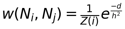 ——– (4)
Z is a normalization constant, and h is the filtering parameter, where
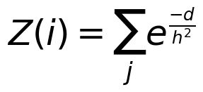 —— (5)
Algorithm 1: Non-Local Means (NLM) Filter
Input:
Image I with noisy pixel intensities
Patch size N
Search window size S
Filter parameter h
Gaussian kernel standard deviation σ
Output:
Filtered image NLM(I)
Initialize an empty image NLM (I) with the same size as the input image I.
For each pixel i in the input image I: a. Define a search window W(i) around the pixel i with size S. b. Iterate through each patch j in the search window W(i):
Calculate the Euclidean distance d between patches I (Ni),and I (Nj) using Equation (3).
Calculate the weight w (Ni, (Nj) for patch j using Equation (4). c. Normalize the weights by dividing each weight w(Ni, Nj) by Z(i), which is the sum of all weights within the search window W(i), calculated using Equation (5). d. Compute the filtered pixel intensity for pixel i using Equation (1), where the intensity is the weighted average of the intensities of neighboring pixels within the search window W(i). e. Assign the filtered pixel intensity to the corresponding pixel in NLM(I).
Return the filtered image NLM(I).
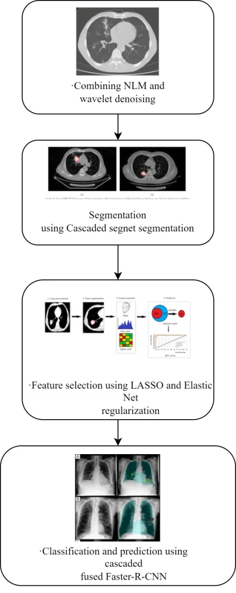
Figure 1 Flow diagram
NLM Denoising Approaches
Several NLM variants have been investigated for medical-image denoising. Fast NLM approaches aim to reduce computational cost. Adaptive variants change the search window, patch size or weighting function according to image noise and local structure. Other approaches modify how similarity and weighting are estimated. These choices can improve the balance between noise reduction and edge preservation, but computational expense remains an important consideration. The appropriate variant depends on the image characteristics and the intended analysis.
Medical images contain repeated patch patterns as well as anatomical features that must remain distinguishable. NLM settings therefore need to balance SNR improvement against bias and oversmoothing. The background discussion notes that excessive smoothing can affect homogeneous regions and that some formulations lack a dedicated acceleration mechanism. It also refers to diffusion-weighted and diffusion-tensor imaging as examples from the broader medical-imaging literature. Those examples should be distinguished from the chest CT collection identified for this study.
Wavelet Denoising
A discrete wavelet transform decomposes an image into an approximation subband and detail subbands at different orientations and resolutions. The detail bands represent horizontal, vertical and diagonal information. Scaling coefficients form the approximation component, while wavelet coefficients describe detail. The manuscript also discusses an undecimated transform, in which the number of coefficients remains constant across scales. This representation supports analysis of image structures at several resolutions.
The wavelet coefficients with the largest positive values are shown in the chart’s boldest hue. HLi, LHi, and HHi detail subbands, whereas big negative values are represented by the darkest hue. The wavelet transform has several desirable qualities as a denoising representation:
Multi-resolution, whereby images of varying sizes are examined at their most suitable resolutions
Most of wavelet coefficients have small absolute values, a property known as “sparsity.”
Large wavelet coefficients are seen around image edges, which may be used for edge detection.
The “edge” coefficients inside each sub band have a tendency to cluster together geographically.
Scale-invariant edge development – coefficients representing image edges tend to be preserved across different zoom levels
Many denoising applications in medical imaging utilize wavelets. The typical method is:
Compute the discrete wavelet transform.
Apply a noise-reduction or thresholding operation to the wavelet coefficients.
Use the inverse wavelet transform to reconstruct the denoised image.
We will discuss a few exceptions to this rule, including magnetic resonance imaging (MRI), but for the most part the scaling coefficients are not changed. In order to estimate the noise-free component of a given wavelet coefficient, wavelet shrinking drastically reduces the coefficients that reflect noise while retaining the coefficients that are more likely to represent the underlying signal or image discontinuities. Wavelet coefficient at location k, orientation D, and resolution 2j(1≤j≤j) is written as wk,jD. Only when absolutely necessary will we provide size and orientation indices. Supposing an additive noise model adequately describes all wavelet bands.
wk=yk+nk ——- (6)
Where yk is the mysterious noiseless signal component and nk is a free-form noise input. Estimators for wavelet shrinking may be summarized as
yk=Rkwk 0≤Rk≤1 ——- (7)
When wk is assumed to represent pure noise, Rk should be close to zero, and when wk represents a real signal or image discontinuity, Rk should be close to one (where Rk represents a variety of compression factors). Standard wavelet thresholding rules (Rk) are provided when a threshold value T is determined. For hard thresholding: . Background noise in MRIs may be reduced with the use of soft thresholding, which was originally used in the medical imaging industry.
Denoising techniques based on wavelets have been developed and used in medical imaging within a Bayesian context. Specifically, Rk=σk2/(σk2+σn2), where σn is the standard deviation of the noise and σk are two instances of Bayesian wavelet domain estimators of the type (2)where is the estimate of the signal’s standard deviation (within a particular local window centered at point k). Not very long ago, a similar but more nuanced strategy was described in. When the wavelet coefficients are considered to be independent of noise, other approaches define Rk as the probability that the coefficient at location k represents a significant signal component. Models based on hidden Markov trees and associated methods are covered.
Algorithm 2 wavelet denoising
Input: Noisy image
Output: Denoised image
Perform the discrete wavelet transform (DWT) on the noisy image.
Estimate the local standard deviation of the noise, σn2.
For each wavelet coefficient wkat location k, orientation D, and resolution 2^j (1 ≤ j ≤ j):
a. Calculate, within a sliding window centered on k, an approximation of the signal’s standard deviation, σk2.
b. Calculate the threshold factor, Rk, using the Bayesian wavelet domain estimator:
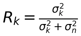
c. Apply soft thresholding to the coefficient using the threshold factor:
wk = Rk * wk
Apply the inverse discrete wavelet transform (IDWT) on the updated coefficients in order to reconstruct the denoised image.
Output the denoised image.
Cascaded SegNet Segmentation
After denoising the data, we apply Cascaded segnet segmentation to segment the image. Figure 2 displays a semantic segmentation model that can extract detailed features from full-sized images. The retrained SegNet’s parameters are fine-tuned with the use of manually labeled images of tumor locations. After the SegNet model is finished, it is put to use in testing by creating tumor segmentation masks from unlabeled images. Due to its few parameters, minimal processing needs, and straightforward end-to-end training, SegNet networks have gained popularity over other forms of deep learning networks. Since U-Net encoders transmit their whole feature maps to their up-sampling decoders, where they are concatenated to form decoder feature maps, these networks demand a lot of memory. In contrast, SegNet networks just reuse pooling indices, which results in reduced memory requirements.
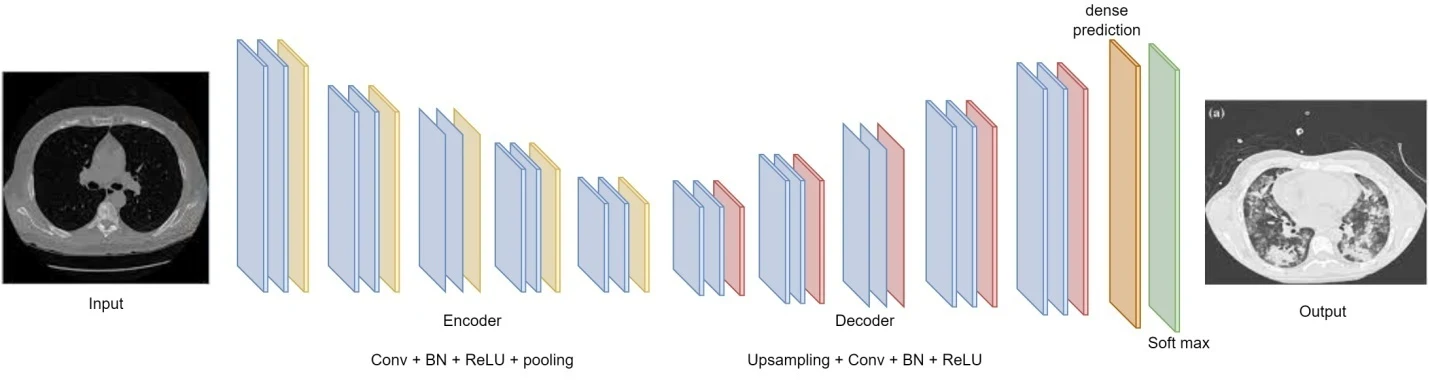
Figure 2: Cascaded segnet SegNet architecture
The primary inspiration from Fully Convolutional Network (FCN) employed in our network design was to convert the VGG-16 fully connected layers into convolutional layers. This results in a decrease from 134M to 14.7M parameters in the SegNet encoder network while maintaining the quality of the feature maps at the deepest outputs of the encoder. A comprehensive feature map with retained spatial information may be generated by the classification net as a result.
The SegNet uses a pixel-by-pixel classification layer after going through an encoding (down sampling) and decoding (up sampling) process. The VGG16 network’s first 13 convolutional layers are functionally equivalent to encoder path layers. The decoder network contains an exact replica of the encoder’s 13 convolutional layers. After the last decoder layer, the data is sent to a multi-class soft-max classifier, which then assigns probabilities to each pixel based on its class.
In the encoder’s final output path, each of the five convolution blocks undergoes a max-pooling operation with a stride of 2 and a window size of 2 by 2. Each convolutional block incorporates batch normalization, element-wise rectified linear nonlinearity (ReLU), and multiple layers of 3 3 convolution. Two of the convolution blocks have two layers, while the other three each have three. The decoder follows a route that is identical to that of the encoder, except that the up sampling process replaces the max-pooling step. The preceding layer’s output and the maximum pooling indices from the relevant encoding layer are both inputs to the up sampling procedure. Each pixel is given a label by a soft-max classifier layer that receives the high-dimensional feature representation generated by the final decoder. Please visit 3n. When training is complete, the soft-max classifier produces an image where each pixel has a probability value, and this image is represented by a K channel, where K is the number of target classes.
Feature Selection Using LASSO
After segmentation, we apply the LASSO and Elastic Net regularization techniques to choose features. To approximate the composite function h (•) at the location x, we first build the following model:
 —— (8)
For if L > 0, then The hL,x(y), Both the smooth function loss (•) and the non-smooth penalty fl (•) are stated in terms of the first-order Taylor expansion at x (containing all terms in the square brackets). Because the regularization factor 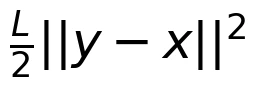 prevents y from deviating too far from x, the model may be a good approximation to h(y) near to x. The following gradient-descent-like approach may be developed using the model in (4) to solve problem (1):
 —— (9)
for a good, solid, and well-chosen {Li}. The technique in (5) has been demonstrated to converge at a rate of o(1/k), and may be accelerated even further to 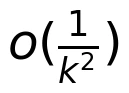 . It is possible to develop the accelerated technique through a lengthy chain of steps called the “estimate sequence”. We provide Nesterov’s technique for solving (9) using the methodology given in eq (10), which makes the presentation rather straightforward. Two sequences, xi (the series of approximate solutions) and s(the sequence of search sites), form the backbone of Nesterov’s approach. The candidate location si is the affine intersection of xi-1 andxi, as
si=xi+βi(xi-xi-1) —— (10)
, where βi is a well-chosen coefficient. As the minimize of hLi,si(y), the approximation Xi+1 is found:
 ——– (11)
Where Li is obtained using a line search using the Armijo-Goldstein technique, and Li ought to be suitable for Si. Algorithm 1 details the procedure for solving (12). The following global convergence result may be established using the evidence presented in:
 ——– (12)
if L is the Lipschitz continuous gradient of the smooth convex loss function loss(•), then X* is the optimal solution to (12).
Algorithm 3 LASSO
Input: Initial solution x0, Lipschitz constant L, convergence tolerance ε
Output: Solution x*
Set i = 0, Li = L, xi = x0, xi-1 = x0
Repeat until convergence: a. Calculate the search site si using the affine intersection: si=xi+βi(xi-xi-1), where βi is a well-chosen coefficient (e.g., βi = i / (i + 3))
b. Perform a line search to determine the appropriate Li for si using the Armijo-Goldstein technique.
c. Update the approximation xi+1 by minimizing the model function
d. Update si=xi+βi(xi-xi-1)
If the stopping criteria are met . Otherwise, go to step 2.
Output the solution x*.
Elastic Net Regularisation
To address difficulties in high-dimensional feature selection, Elastic Net (EN) regularization was created as a version of multiple linear regression techniques. To improve prediction accuracy by automated variable selection and ongoing shrinkage, the EN makes use of two penalty terms (L1-norm and L2-norm). This approach, analogous to a stretchable fishing net, only keeps the most important information (“big fish”) and throws away the rest. The linear regression equation for estimating the response variable y is y=β0+β1x1+…+βpxp, if we have p predictors. The coefficients (β=[β0,…,βp]) are obtained by minimizing the sum of squares of the error residuals Equation 13. Coefficients are determined not by the SSE but by minimizing the L function equation 14. If there are more features than observations:
SSE=||Y-Xβ||2 —— (13)
 ——– (14)
The L1 and L2 norm terms in the objective control different aspects of coefficient shrinkage. Equations (14) and (15) give the penalty expression and squared-norm relationship used in the manuscript.
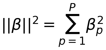 ——- (15)
The weighting parameters α and ρ determine the strength and balance of the penalties. Their selection affects the model output and is therefore part of model tuning. At ρ = 1, the stated formulation reduces to a LASSO-type penalty. At ρ = 0, it becomes a ridge-type penalty. Elastic Net combines these two forms of shrinkage and can retain groups of correlated predictors while controlling model complexity. This provides a feature-selection option where the number of candidate features is large relative to the available observations.
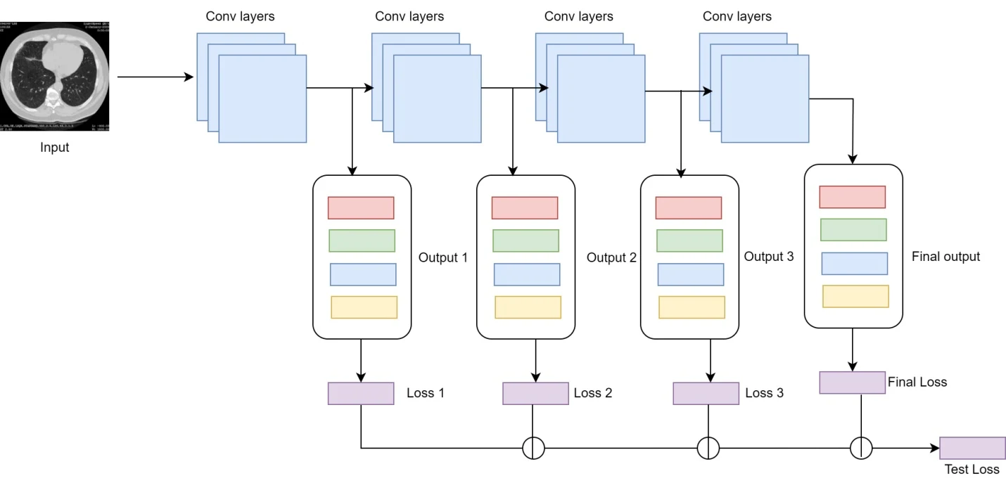
Figure 3: Elastic Net architecture
Algorithm 4 Elastic Net
Input: Predictor matrix X (size n x p), response variable vector Y (size n), regularization parameters α and ρ
Output: Coefficient vector β (size p)
Initialize the coefficient vector (β=[β0,…,βp]) as all zeros or with an initial guess.
At each iteration, calculate the fitted values ŷ = Xβ.
b. Calculate the residuals vector r = Y – ŷ.
Update the coefficient vector β by minimizing the objective function: SSE=||Y-Xβ||2
If ρ = 1, perform LASSO regression:
If ρ = 0, perform ridge regression:
Update the weighting variables α and ρ if necessary.
Output the final coefficient vector β.
Cascaded Fused Faster R-CNN Classification
After feature selection, the workflow uses Cascaded Fused Faster R-CNN for lung-image classification. A CNN extracts image features, and a region proposal network (RPN) identifies candidate regions. Region-of-interest (ROI) pooling converts the corresponding features to a fixed-size representation. Classification and bounding-box regression then operate on those representations. Figure 4 shows the supplied architecture. The intended application here is image-region analysis and classification.
Object detection seeks both the location and category of an object in an image. Faster R-CNN uses an RPN to generate candidate regions rather than relying on a separate selective-search process. Feature maps support region proposals and subsequent classification. In the described cascaded workflow, successive processing stages refine the candidate representations. The model combines region proposal with Fast R-CNN-style classification and localisation. Texture, edges and other image features contribute to identifying relevant regions, while the proposal stage limits the number of locations requiring later processing.
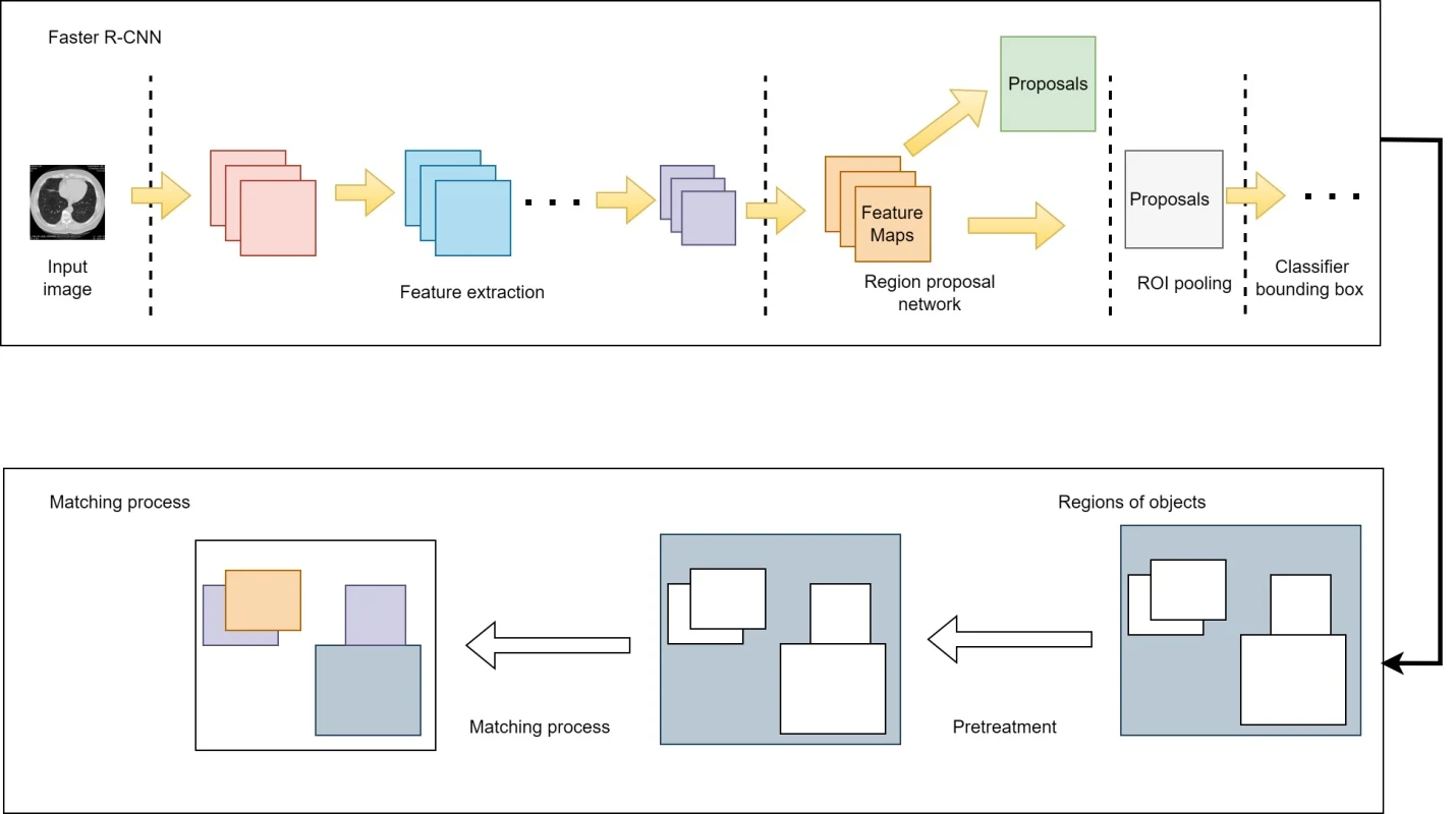
Figure 4: Cascaded fused Faster R-CNN architecture
The architecture uses convolutional feature extraction, an RPN and fully connected prediction components. Feature maps are shared with later stages. The RPN evaluates anchor locations and estimates bounding-box offsets. A classification output distinguishes foreground from background. ROI pooling then uses the proposals and feature maps to construct fixed-size inputs for subsequent prediction layers. The source gives inconsistent layer-count descriptions, so no definitive total is assigned here.
Results and Discussion
The proposed workflow combines image denoising, region segmentation, feature selection and classification. NLM and wavelet processing prepare the images; Cascaded SegNet provides lung-region representations; and LASSO and Elastic Net control the selected features. Cascaded Fused Faster R-CNN supplies the final classification stage. The following tables and figures reproduce the manuscript’s experimental comparisons, including confusion-count measures, classification metrics, image-quality measures and test loss.
Table 2: Performance metrics comparison
Performance metrics | ||||
CNN | ANN | Faster R-CNN | cascaded fused Faster R-CNN | |
True Positives | 1869 | 2154 | 3547 | 4517 |
False Positives | 1024 | 1845 | 2635 | 4157 |
False Negatives | 1854 | 2454 | 3621 | 4517 |
True Negatives | 1035 | 1834 | 3514 | 4821 |
The reported performance of the models is described by the performance measures shown in Table 2. CNN, ANN, Faster R-CNN, and cascaded fused Faster R-CNN are the four models we have here. True positives, false positives, false negatives, and true negatives are all measured. Accurately classified examples are referred to as “true positives,” and they are the focus of this discussion. For example, the cascaded fused Faster R-CNN model achieved 4517 true positive predictions, indicating its ability to accurately detect and classify objects. False positives, on the other hand, represent instances that were incorrectly identified as belonging to the target class. In this scenario, the cascaded fused Faster R-CNN model had 4157 false positive predictions, which suggests that it might have classified some objects incorrectly. False negatives indicate instances that were wrongly classified as not belonging to the target class. For instance, the ANN model had 2454 false negative predictions, implying that it missed a considerable number of instances that should have been classified correctly. Lastly, true negatives represent instances correctly identified as not belonging to the target class. The cascaded fused Faster R-CNN model achieved 4821 true negative predictions, indicating its ability to accurately reject objects that don’t belong to the target class. By analyzing these metrics, we can compare the performance of different models and assess their strengths and weaknesses. It’s important to consider the specific task and context when interpreting these metrics, as they provide a snapshot of the models’ performance on the given dataset.
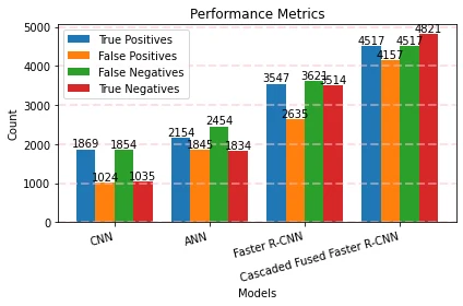
Figure 5: Performance metrics comparison
Figure 5 compares the reported true-positive, false-positive, false-negative and true-negative counts for the four models.
Table 3: Performance metrics comparison
Performance metrics | ||||
CNN | ANN | Faster R-CNN | cascaded fused Faster R-CNN | |
Sensitivity | 0.3636 | 0.4745 | 0.5421 | 0.6354 |
Positive Detection Probability | 0.3818 | 0.4124 | 0.4867 | 0.5314 |
Negative Detection Probability | 0.2153 | 0.3247 | 0.4715 | 0.5124 |
False Discovery Rate | 0.1132 | 0.2457 | 0.3247 | 0.4178 |
The performance metrics in Table 3 offer valuable insights into the effectiveness of different machine learning models. These metrics, including sensitivity, positive detection probability, negative detection probability, and false discovery rate, allow us to evaluate the models’ performance in various aspects. The models’ accuracy in identifying positive cases is measured by their sensitivity, which is also known as recall or true positive rate. The cascaded fused Faster R-CNN model had the maximum sensitivity of 0.6354, indicating a stronger capacity to recognize positive occurrences. The percentage of projected positive cases that are really positive is known as the “positive detection probability”. The cascaded fused Faster R-CNN model also excelled in this metric, with a positive detection probability of 0.5314. On the other hand, negative detection probability measures the models’ ability to accurately detect negative instances out of all the instances predicted as negative. Once again, the cascaded fused Faster R-CNN model outperformed the others with a negative detection probability of 0.5124. The percentage of incorrect positive model predictions is represented by the false discovery rate. The CNN model achieved the lowest false discovery rate of 0.1132, suggesting its superior performance in minimizing false positive predictions.
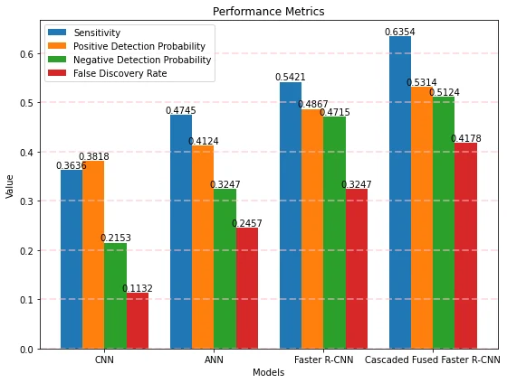
Figure 6: Performance metrics
Different machine learning models’ performance measures are shown in Figure 6. On the x-axis are the names of the models being compared, and along the y-axis are their corresponding performance scores. Each point or mark on the graph corresponds to a specific model and its corresponding value for a particular metric. The position along the y-axis indicates the value of the metric achieved by the respective model. For instance, if the value of a metric is higher, the corresponding point on the graph will be higher on the y-axis.
Table 4: Mean Squared Error and G-Mean comparison
Performance metrics | ||||
CNN | ANN | Faster R-CNN | cascaded fused Faster R-CNN | |
Mean Squared Error | 0.0015 | 0.0034 | 0.0064 | 0.0087 |
G-Mean | 0.2879 | 0.3457 | 0.4321 | 0.5437 |
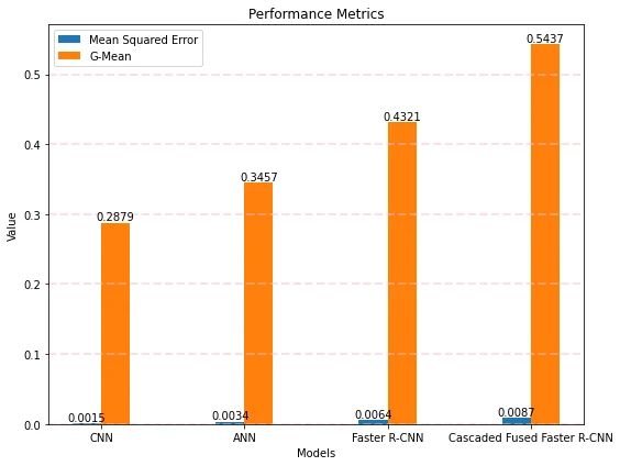
Figure 7: Mean Squared Error and G-Mean comparison
Mean Squared Error (MSE) and G-Mean values are compared across several machine learning models in Figure 7. Model names are shown along the x-axis, while MSE and G-Mean values are shown along the y-axis. The mean squared error (MSE) is a statistic for evaluating the accuracy of a regression model. When MSE is lower, the anticipated and observed values are more in agreement. In the graph, each point or mark on the graph represents the MSE value achieved by a specific model. Lower points on the y-axis indicate models with lower MSE values, indicating superior accuracy in their predictions.
Table 5: PSNR comparison
Performance metrics | ||||
CNN | ANN | Faster R-CNN | cascaded fused Faster R-CNN | |
Peak Signal-to-Noise Ratio | 14.1812 | 15.6478 | 16.9547 | 17.2457 |
Performance metrics for various machine learning models are presented in terms of Peak Signal-to-Noise Ratio (PSNR) values, as shown in table 5. The peak signal-to-noise ratio (PSNR) is a popular measure for judging the accuracy of a signal reconstruction or a signal generation by comparing the two to the original. The ratio between the signal’s highest potential power and the noise power in the reconstruction is calculated. In this scenario, the PSNR values for the models are as follows: CNN: 14.1812, ANN: 15.6478, Faster R-CNN: 16.9547, and Cascaded fused Faster R-CNN: 17.2457. A higher PSNR value indicates a better quality reconstruction, indicating a smaller difference between the original signal and the reconstructed version. Among the models evaluated, the cascaded fused Faster R-CNN model achieved the highest PSNR value of 17.2457. This suggests that it produced a reconstruction with a higher level of fidelity to the original signal compared to the other models.
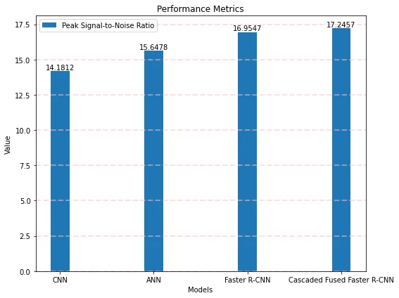
Figure 8: PSNR comparison
Peak Signal-to-Noise Ratio (PSNR) values are compared across several machine learning models in Figure 8. The graph’s x-axis displays the models under consideration, while the y-axis shows the PSNR values attained by each.
Table 6: performance metrics comparison
Performance metrics | ||||
CNN | ANN | Faster R-CNN | cascaded fused Faster R-CNN | |
Accuracy | 0.6818 | 0.7654 | 0.8467 | 0.9657 |
Precision | 0.65 | 0.69 | 0.71 | 0.84 |
Recall | 0.5668 | 0.5987 | 0.6478 | 0.7415 |
F1 score | 0.6841 | 0.7458 | 0.8467 | 0.9847 |
Test accuracy | 0.6915 | 0.7415 | 0.8247 | 0.9874 |
Table 6 reports accuracy, precision, recall, F1 score and test accuracy for CNN, ANN, Faster R-CNN and Cascaded Fused Faster R-CNN. The proposed model’s stated values are 0.9657 accuracy, 0.84 precision, 0.7415 recall, 0.9847 F1 score and 0.9874 test accuracy. Accuracy describes the fraction of correctly classified instances, precision concerns the fraction of predicted positives that are positive, and recall concerns the fraction of actual positives detected. F1 combines precision and recall. The manuscript’s reported values are preserved, but several metrics do not reconcile with one another or with the confusion counts. They therefore should not be treated as a verified, internally consistent estimate of clinical performance.
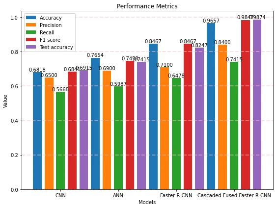
Figure 9: Performance metrics comparison
Metrics indicating the effectiveness of several machine learning models are graphically shown in Figure 9. The graph’s x-axis shows which models are being measured, while the y-axis shows how their performance measures stack up.
Table 7: Test loss comparison
Performance metrics | ||||
CNN | ANN | Faster R-CNN | cascaded fused Faster R-CNN | |
Test loss | 0.0683 | 0.0575 | 0.0417 | 0.0347 |
Table 7 reports test-loss values of 0.0683 for CNN, 0.0575 for ANN, 0.0417 for Faster R-CNN and 0.0347 for Cascaded Fused Faster R-CNN. Lower loss indicates a better fit under the particular loss function used; loss is not inherently a percentage difference or a clinical accuracy measure. The proposed model has the lowest reported test loss in this comparison. The loss function and evaluation protocol would need to be specified fully to support reproducible comparisons.
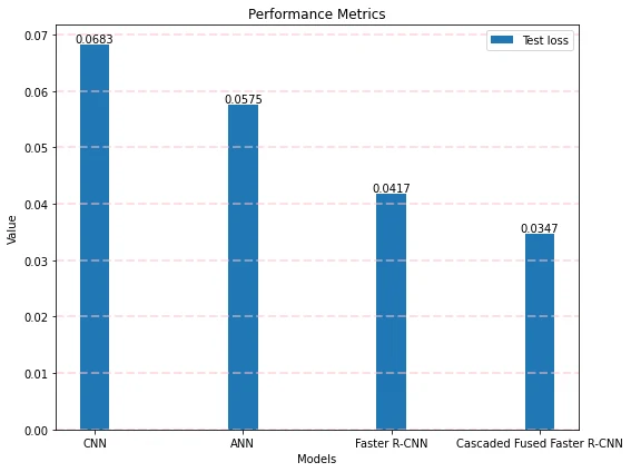
Figure 10: Test loss comparison
Figure 10 illustrates a comparison of test loss values for different machine learning models. Each model’s test loss is shown against its evaluation on a graph, with the models’ names along the x-axis.
Conclusion
This paper examines a Cascaded Fused Faster R-CNN framework for lung-image classification. Its stages combine NLM and wavelet denoising, Cascaded SegNet segmentation, LASSO and Elastic Net feature selection, and region-based classification. Denoising aims to retain important image information while reducing noise. Segmentation supplies lung-region representations for later processing, while regularisation limits the feature space and model complexity. The classification architecture then uses region proposals and pooled features to produce outputs. The manuscript presents comparison tables and figures for this workflow. Further work would require a clearly documented evaluation protocol and reconciliation of the reported metrics before independent performance claims could be assessed.
References
Bartholomai, J. A., & Frieboes, H. B. (2018). Lung Cancer Survival Prediction via Machine Learning Regression, Classification, and Statistical Techniques. 2018 IEEE International Symposium on Signal Processing and Information Technology (ISSPIT). doi:10.1109/isspit.2018.8642753
Carioli, G., Malvezzi, M., Bertuccio, P., Boffetta, P., Levi, F., La Vecchia, C., & Negri, E. (2021). European cancer mortality predictions for the year 2021 with focus on pancreatic and female lung cancer. Annals of Oncology, 32(4), 478–487. doi:10.1016/j.annonc.2021.01.006
Doppalapudi, S., Qiu, R. G., & Badr, Y. (2021). Lung cancer survival period prediction and understanding: Deep learning approaches. International Journal of Medical Informatics, 148, 104371. doi:10.1016/j.ijmedinf.2020.104371
Duruisseaux, M., Martínez-Cardús, A., Calleja-Cervantes, M. E., Moran, S., Castro de Moura, M., Davalos, V., … Esteller, M. (2018). Epigenetic prediction of response to anti-PD-1 treatment in non-small-cell lung cancer: a multicentre, retrospective analysis. The Lancet Respiratory Medicine. doi:10.1016/s2213-2600(18)30284-4
Faisal, M. I., Bashir, S., Khan, Z. S., & Hassan Khan, F. (2018). An Evaluation of Machine Learning Classifiers and Ensembles for Early Stage Prediction of Lung Cancer. 2018 3rd International Conference on Emerging Trends in Engineering, Sciences and Technology (ICEEST). doi:10.1109/iceest.2018.8643311
Gu, Q., Feng, Z., Liang, Q., Li, M., Deng, J., Ma, M., … Rong, P. (2019). Machine learning-based radiomics strategy for prediction of cell proliferation in non-small cell lung cancer. European Journal of Radiology, 118, 32–37. doi:10.1016/j.ejrad.2019.06.025
Haarburger, C., Weitz, P., Rippel, O., & Merhof, D. (2019). Image-Based Survival Prediction for Lung Cancer Patients Using CNNS. 2019 IEEE 16th International Symposium on Biomedical Imaging (ISBI 2019). doi:10.1109/isbi.2019.8759499
He, T., Guo, J., Chen, N., Xu, X., Wang, Z., Fu, K., … Yi, Z. (2019). MediMLP: Using Grad-CAM to Extract Principal Variables for Lung Cancer Postoperative Complication Prediction. IEEE Journal of Biomedical and Health Informatics, 1–1. doi:10.1109/jbhi.2019.2949601
Heuvelmans, M. A., van Ooijen, P. M. A., Ather, S., Silva, C. F., Han, D., Heussel, C. P., … Oudkerk, M. (2021). Lung cancer prediction by Deep Learning to identify benign lung nodules. Lung Cancer, 154, 1–4. doi:10.1016/j.lungcan.2021.01.027
Huang, P., Lin, C. T., Li, Y., Tammemagi, M. C., Brock, M. V., Atkar-Khattra, S., … Lam, S. (2019). Prediction of lung cancer risk at follow-up screening with low-dose CT: a training and validation study of a deep learning method. The Lancet Digital Health. doi:10.1016/s2589-7500(19)30159-1
Jayaraj, D., & Sathiamoorthy, S. (2019). Random Forest based Classification Model for Lung Cancer Prediction on Computer Tomography Images. 2019 International Conference on Smart Systems and Inventive Technology (ICSSIT). doi:10.1109/icssit46314.2019.8987772
Kumar, D., Sankar, V., Clausi, D., Taylor, G. W., & Wong, A. (2019). SISC: End-to-End Interpretable Discovery Radiomics-Driven Lung Cancer Prediction via Stacked Interpretable Sequencing Cells. IEEE Access, 7, 145444–145454. doi:10.1109/access.2019.2945524
Luo, Y., McShan, D., Ray, D., Matuszak, M., Jolly, S., Lawrence, T., … El Naqa, I. (2018). Development of a Fully Cross-Validated Bayesian Network Approach for Local Control Prediction in Lung Cancer. IEEE Transactions on Radiation and Plasma Medical Sciences, 1–1. doi:10.1109/trpms.2018.2832609
Malvezzi, M., Carioli, G., Bertuccio, P., Boffetta, P., Levi, F., La Vecchia, C., & Negri, E. (2017). European cancer mortality predictions for the year 2017, with focus on lung cancer. Annals of Oncology, 28(5), 1117–1123. doi:10.1093/annonc/mdx033
Pati, J. (2019). Gene Expression Analysis for Early Lung Cancer Prediction Using Machine Learning Techniques: An Eco-Genomics Approach. IEEE Access, 7, 4232–4238. doi:10.1109/access.2018.2886604
Petousis, P., Winter, A., Speier, W., Aberle, D. R., Hsu, W., & Bui., A. A. T. (2019). Using Sequential Decision Making to Improve Lung Cancer Screening Performance. IEEE Access, 1–1. doi:10.1109/access.2019.2935763
PR, R., Nair, R. A. S., & G, V. (2019). A Comparative Study of Lung Cancer Detection using Machine Learning Algorithms. 2019 IEEE International Conference on Electrical, Computer and Communication Technologies (ICECCT). doi:10.1109/icecct.2019.8869001
Raoof, S. S., Jabbar, M. A., & Fathima, S. A. (2020). Lung Cancer Prediction using Machine Learning: A Comprehensive Approach. 2020 2nd International Conference on Innovative Mechanisms for Industry Applications (ICIMIA). doi:10.1109/icimia48430.2020.9074947
Shukla, R. S., & Aggarwal, Y. (2018). Nonlinear Heart Rate Variability based artificial intelligence in lung cancer prediction. Journal of Applied Biomedicine, 16(2), 145–155. doi:10.1016/j.jab.2017.12.002
Suresh, S., & Mohan, S. (2020). ROI-based feature learning for efficient true positive prediction using convolutional neural network for lung cancer diagnosis. Neural Computing and Applications. doi:10.1007/s00521-020-04787-w
Thallam, C., Peruboyina, A., Raju, S. S. T., & Sampath, N. (2020). Early Stage Lung Cancer Prediction Using Various Machine Learning Techniques. 2020 4th International Conference on Electronics, Communication and Aerospace Technology (ICECA). doi:10.1109/iceca49313.2020.9297576
Van Timmeren, J. E., Leijenaar, R. T. H., van Elmpt, W., Reymen, B., Oberije, C., Monshouwer, R., … Lambin, P. (2017). Survival prediction of non-small cell lung cancer patients using radiomics analyses of cone-beam CT images. Radiotherapy and Oncology, 123(3), 363–369. doi:10.1016/j.radonc.2017.04.016
Wang, X., Chen, H., Gan, C., Lin, H., Dou, Q., Tsougenis, E., … Heng, P.-A. (2019). Weakly Supervised Deep Learning for Whole Slide Lung Cancer Image Analysis. IEEE Transactions on Cybernetics, 1–13. doi:10.1109/tcyb.2019.2935141
Weissfeld, J. L., Lin, Y., Lin, H.-M., Kurland, B. F., Wilson, D. O., Fuhrman, C. R., … Diergaarde, B. (2015). Lung Cancer Risk Prediction Using Common SNPs Located in GWAS-Identified Susceptibility Regions. Journal of Thoracic Oncology, 10(11), 1538–1545. doi:10.1097/jto.0000000000000666
Yu, D., Liu, Z., Su, C., Han, Y., Duan, X., Zhang, R., … Xu, S. (2019). Copy number variation in plasma as a tool for lung cancer prediction using Extreme Gradient Boosting (XGBoost) classifier. Thoracic Cancer. doi:10.1111/1759-7714.13204
Zhang, L., Chen, B., Liu, X., Song, J., Fang, M., Hu, C., … Tian, J. (2018). Quantitative Biomarkers for Prediction of Epidermal Growth Factor Receptor Mutation in Non-Small Cell Lung Cancer. Translational Oncology, 11(1), 94–101. doi:10.1016/j.tranon.2017.10.012
Cite This Work
To export a reference to this article please select a referencing stye below:

Academic Master Education Team is a group of academic editors and subject specialists responsible for producing structured, research-backed essays across multiple disciplines. Each article is developed following Academic Master’s Editorial Policy and supported by credible academic references. The team ensures clarity, citation accuracy, and adherence to ethical academic writing standards
Content reviewed under Academic Master Editorial Policy.