Cascaded Recurrent Fuzzy Filters for Alzheimer MRI and PET Classification

Abstract

Alzheimer’s disease (AD) is a progressive neurodegenerative condition characterized by cognitive decline and memory loss. Computer-Aided Diagnosis (CAD) has become a potent instrument for its early and accurate detection thanks to developments in the biomedical area. Positron Emission Tomography (PET), Magnetic Resonance Imaging (MRI), and Computed Tomography (CT) data are integrated in this multimodal technique to improve the stability and robustness of the diagnosis. The CAD process initiates with image preprocessing, as collected images often contain noise that can block accurate segmentation and classification. Various enhancement techniques, including Local Entropy Weighted Histogram Equalization (LEWHE) and guided image denoising using an adaptive Salp Swarm Optimization algorithm (ASSO), are employed alongside geometric transformations, image augmentation, noise reduction, and grayscale conversion. These techniques refine the dataset, setting the stage for precise segmentation and classification. For segmentation and classification, the study introduces a novel SC-GRU: CDREFM_Net (Sine Cosine based GRU classification with Cascaded Dilated Recurrent Entropy fuzzy with Mask Region Convolutional Neural Network (MRCNN)). This architecture uses the Chaos-Infused Chimp Sine Cosine (CICSC) algorithm for semantic segmentation, offering high-level feature performance. CDREFM_Net adopts multiple kernel sizes and a Recurrent Fuzzy Filter (RFF) to enhance feature learning through dilation and entropy. Additionally, the Gated Recurrent Unit (GRU) is employed for classification, capturing sequential dependencies in the data. The proposed model has been successfully implemented using MATLAB, and it demonstrates outstanding performance with a remarkable accuracy rate of 99%.

Keywords: Alzheimer’s Disease; LEWHE; CICSC; ASSO; GRU; RFF.

Introduction

AD is a severe neurological condition that affects millions of people and leaves them feeling uncertain and hopeless. It is a cruel enemy that slowly destroys a person’s most priceless memories, cognitive abilities, and social skills, leaving a path of broken lives and loss in its wake [1]. AD is a severe ailment that affects an estimated 6.5 million people in the United States alone who are 65 years of age and older [2,3]. The majority of people affected are 75 years of age or older, bearing the heavy burden of a sickness that threatens not only their capacity to function in the present but also erases their past [4]. With an estimated 60% to 70% of the approximately 55 million people suffering from memory worldwide, AD throws an even larger net of misery beyond the borders of the United States [5]. A secret epidemic that destroys both individuals and families on a global scale. The gradual loss of recent memories, with conversations and events passing through the fingers of recall like sand grains, is usually where AD starts. Even more depressingly, there is no known treatment for AD [6,7]. In Alzheimer’s topographic pattern, initial alterations occur in the medial temporal lobe, including the entorhinal cortex, perirhinal cortex, and hippocampus [26].

Figure 1: Areas impacted by AD [26]

Recent developments in artificial intelligence and medical imaging have created new possibilities for studying, identifying, and maybe treating AD [8]. An effective tool in this effort is deep learning, a branch of artificial intelligence that holds the promise of drawing vital conclusions from images of the body and potentially revolutionising how we treat this fatal disease [9]. Deep learning models have already had outstanding success in a number of medical imaging fields, including mammography, X-rays, MRI images, CT scans, and microscopy. These models have the potential to go much farther, enabling the classification of various phases of memory [10]. They are not just capable of detecting the existence of AD. This is especially important in the case of Mild Cognitive Impairment (MCI), a highly risky stage at which 10% to 16% of people annually experience a rapid progression to AD [11]. The diversity of MCI is what makes it so distinctive; some people even stabilize or even return to health. MRI is developing as a significant technique for this, and important biomarkers are required for predicting the change from MCI to Alzheimer’s [12]. In the rapidly advancing field of biomedicine, CAD has emerged as a powerful tool for AD detection. Multi-task modeling, incorporating various modalities like MRI, CT, and PET scans, enhances diagnostic accuracy [13]. This approach offers superior robustness, progression tracking, and stability, making it a promising method for Alzheimer’s diagnosis. Figure 2 illustrates a visual comparison between individuals with normal brain function and those affected by Alzheimer’s disease.

Figure 2: Comparison between Normal and Alzheimer’s Disease [27]

Magnetic resonance images are particularly well-suited for clinical applications because they provide a plethora of multi-modal data regarding the anatomy and physiology of the brain [14]. The deep learning methods of choice for precisely identifying and making predictions from high-level data retrieved from medical pictures are convolutional neural networks (CNN). CNNs are the cornerstone of deep learning applications in medical imaging due to their efficacy in image processing and classification [15]. Despite how encouraging these improvements may seem, they are not without difficulties and restrictions. Existing deep learning and machine learning models frequently rely on training from scratch, which is a time- and resource-consuming procedure. Furthermore, overfitting is a serious issue that can negatively impact the performance of these models as a whole due to the intricate tuning of various parameters during model training. Despite these challenges, the combination of deep learning and medical imaging offers an exciting glimpse into a future when AD might not be the overpowering threat at present.

The primary contributions of this research are:

To Improve Image Quality: To enhance the quality of collected biomedical images, novel techniques like LEWHE with an AWDO algorithm and Guided filter-based image denoising using an ASSO algorithm are proposed. These methods contribute to creating a refined dataset for subsequent segmentation and classification.

To Advance Multi-Modal Diagnosis: By considering multiple modalities, including MRI, CT, and PET, this research contributes to a holistic and robust Alzheimer’s diagnosis approach. The incorporation of multi-modal data improves robustness, progression-detection performance, and stability in the diagnosis process.

To Introduce a Novel Segmentation Model: The introduction of CDREFM_Net with CICSC contributes to the field by providing an advanced semantic segmentation model. This model leverages multiple feature learning, dilation, entropy, and recurrent fuzzy filters to achieve high-level feature performance in AD image segmentation.

To Enhance Classification Accuracy: Utilizing GRU for classification in conjunction with the proposed segmentation model, this research contributes to improved classification accuracy in AD diagnosis. The integration of GRU further refines the diagnostic capabilities of the CAD system.

The following is the arrangement of the remaining sections: The research and literature reviews that are relevant to the topic are covered in Section 2. The suggested framework is talked about in Section 3. Section 5 concludes this study, while Section 4 describes the outcomes that were recorded.

Literature Review

In 2022, Palacios-Navarro et al. [16] assessed the efficacy of an Activities of Daily Living (ADL)-based task for detecting cognitive impairment in AD patients. Their study involved twenty-four participants, including 12 individuals with AD and 12 healthy controls. These participants underwent the ADL-based intervention twice, with a 3-week gap between assessments. Cognitive function was evaluated using the MEC-35 test before and after the interventions. In 2021, Li et al. [17] delved into EEG analysis for early AD diagnosis. They focused on latent factors’ role in characterizing cognitive impairment and employed a variational auto-encoder to extract disease-related features from EEG data, particularly emphasizing differences in the theta frequency band. Their study also incorporated a Takagi-Sugeno-Kang fuzzy classifier, achieving an impressive accuracy rate of 98.10% in identifying neurological dysfunction. The topic of incorporating machine learning into dementia diagnosis was taken on by Mccombe et al. [18] in 2022, who focused on the importance of assessment time. In order to choose cognitive and functional assessment items for AD diagnosis as efficiently as possible, they used a variety of feature selection strategies. Additionally, they created a user-friendly sandbox tool that enables stakeholders and physicians to alter dementia diagnostic tests in order to increase speed and accuracy. In order to obtain slice-wise volumetric characteristics from the left and right hippocampi, Basher et al. [19] employed structural MRI data in 2021, concentrating on the diagnosis of AD. Convolutional neural networks (CNN) and deep neural networks (DNN) were used in conjunction, and Hough-CNN was used for automatic hippocampus localization.

Gao et al. [20] used cutting-edge medical imaging methods like MRI and PET in 2022 to improve AD diagnosis. Their novel strategy combined a Pathwise Transfer Dense Convolution Network (PT-DCN) with a Task-Induced Pyramid and Attention Generative Adversarial Network (TPA-GAN). By combining pyramid convolution, attention modules, and disease classification within a GAN architecture, TPA-GAN successfully produced missing PET data from MRI. To address the growing worry over the occurrence of AD, Liu et al. [21] created the AD Conversion Risk Estimation System (CRES) in 2023. A Brain Age Estimation (BAE) module, an AD conversion risk estimator, and an MRI-based feature extractor were all included in CRES. Using MRI-derived age and trained on 634 normal controls and tested on 462 ADNI dataset participants, CRES successfully distinguished between NC, sMCI, pMCI, and AD groups. In 2021, Zhao et al. [22] addressed the pressing need for long-term AD progression prediction. Their novel framework combined a 3D multi-information generative adversarial network (mi-GAN) for forecasting future individual brain MRI images with a 3D DenseNet-based multi-class classification network optimized with focal loss. In 2020, Brand et al. [23] introduced a groundbreaking approach to address the escalating public health concern of AD. Their Joint Multi-Modal Longitudinal Regression and Classification method leveraged clinical data, including genetic information and brain scans from the ADNI cohort. By simultaneously addressing cognitive status identification and elucidating underlying biological mechanisms, their approach provided a rigorous solution to a complex non-smooth optimization problem.

Ashtari-Majlan et al. [24] emphasized the need of detecting moderate cognitive impairment (MCI), which is a precursor to AD, in 2022. In order to distinguish between stable and progressive MCI, their method made use of a multi-stream deep convolutional neural network and patch-based imaging data. By comparing MRI images of AD patients with those of cognitively normal subjects, they identified distinct anatomical features and used them to extract patches. These patches were then processed through their multi-stream CNN, and the model’s performance was further enhanced by fine-tuning with progressive and stable MCI data. In 2019, Ahmed et al. [25] acknowledged the growing popularity of deep learning in AD diagnosis, particularly for multimodal approaches. However, they noted the challenges in data collection and safety concerns. Their study specifically focused on structural MRI (sMRI) for AD diagnosis, aiming to boost accuracy to match state-of-the-art methods, address overfitting, and identify distinctive brain landmarks, particularly the left and right hippocampus regions. Table 1 illustrates research gaps similarity to cutting-edge approaches.

Table 1: Research gaps

Problem Statement

Millions of people throughout the world suffer with AD, an advanced neurological ailment. The key to effective management is an early, accurate diagnosis. The diagnosis of AD is aided by MRI, which reveals structural brain abnormalities and biomarkers. Manual interpretation, however, requires a lot of time and is unpredictable and subjective. For precise MRI-based brain structure segmentation and classification, automated methods are required. The classification of AD comes with difficulties, including hurdles for early identification of minor cognitive changes, the incorporation of various data types including MRI and genomics, the management of unbalanced datasets, and avoiding overfitting in deep learning models [1,5]. Finding significant characteristics and guaranteeing model repeatability across many datasets are major issues. Complexity is increased by the ethical issues brought on by the use of private medical information and the requirement for clinical validation. While data preprocessing was the main focus of earlier research, the present work concentrates on the important phases of segmentation and classification. Multimodal cooperation, solid data, cutting-edge machine learning methods, and ongoing research efforts are required to address these complexities [18].

Proposed Methodology

AD is a progressive neurological condition characterized by cognitive decline, memory loss, and difficulty completing daily tasks. Common problems associated with Alzheimer’s include confusion, disorientation, difficulty in communication, and eventual loss of independence in daily activities. The rapid advancements in biomedicine have led to the emergence of CAD as an effective tool for Alzheimer’s disease detection. Multi-task modeling, encompassing various modalities like MRI, CT, and PET scans, enhances diagnostic accuracy, robustness, and progression tracking capabilities. This study introduced an optimized MRCNN framework utilizing cascaded dilated recurrent fuzzy filters, enhancing Alzheimer’s disease segmentation and classification. Figure 3 depicts the overall proposed architecture.

Data Collection

The dataset used for this study is the LONI Image Data Archive (IDA) dataset, is a collection of medical imaging and related data that researchers can access and utilize for various studies and investigations. It provides a valuable resource for research in fields such as neuroscience and neuroimaging. It consists of total of 7,190 images. These images are divided into two modalities: MRI and PET, each containing 3,595 images. The dataset focuses on two distinct classes: AD and Cognitive Normal (CN). For the training and testing split, an 80-20 ratio is employed. This means that 80% of the dataset, which corresponds to 5,752 images (2,876 from each class), is used for training the machine learning or deep learning models. The remaining 20% of the dataset, totaling 1,438 images (719 from each class), is reserved for testing the models to evaluate their performance. By ensuring that the models are trained on a sizable piece of the data while keeping a separate set for objective evaluation, this partitioning method makes it easier to evaluate the models’ accuracy and generalization skills.

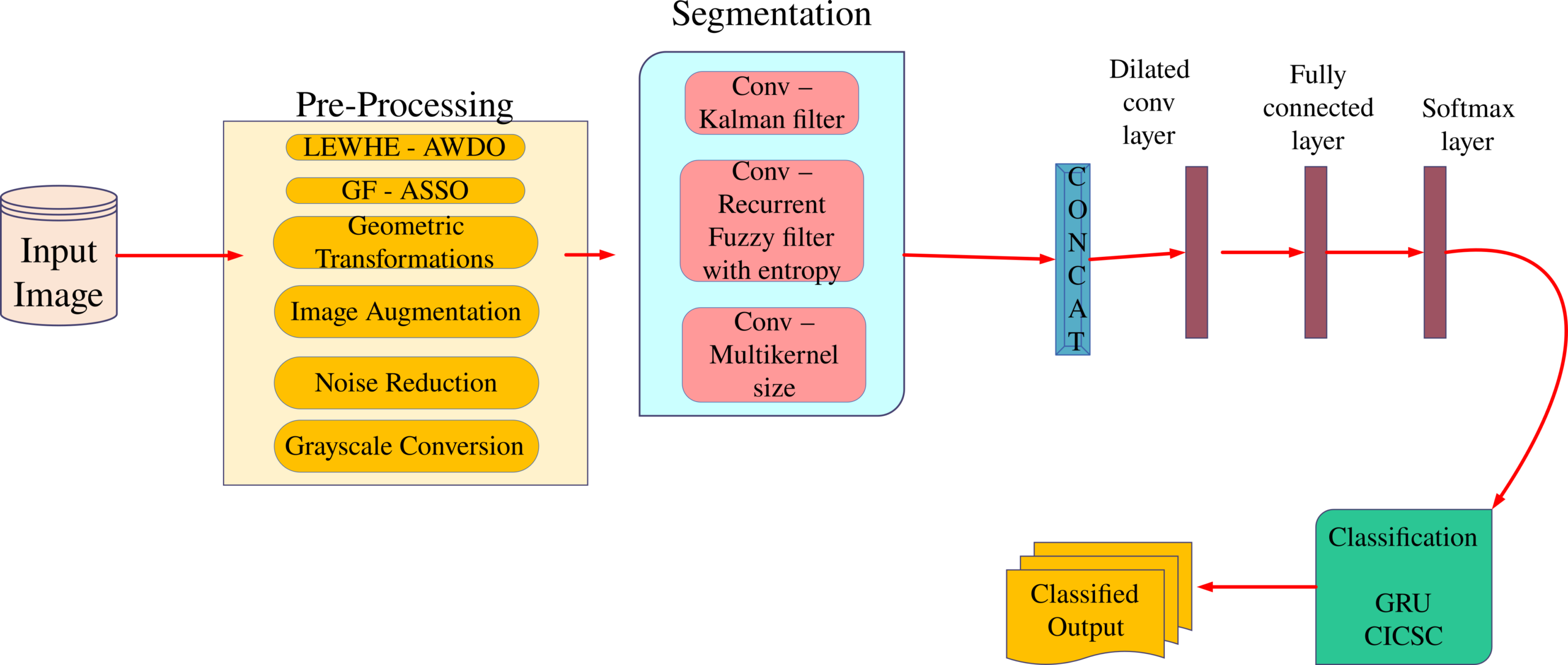
Figure 3: Overall Proposed Architecture

Pre-Processing

Pre-processing in this research involves geometric transformations, image augmentation, noise reduction, grayscale conversion, LEWHE using an adaptive wind-driven optimization algorithm, and guided filter-based image denoising using an adaptive salp swarm optimization algorithm.

LEWHE

LEWHE is a valuable technique in the realm of AD detection, particularly for enhancing the contrast and clarity of MRI brain images. This approach breaks down the input image into non-overlapping sub-regions and independently equalizes the histograms of each sub-region. The key innovation lies in the utilization of local entropy, which determines the weight of each pixel’s contribution to the overall histogram. This process yields a refined image that significantly aids in the precise and efficient detection of AD. The algorithm encompasses several critical steps, including sub-region division, local entropy computation, local entropy-weighted histogram (LEWH) calculation, optimal threshold-based segmentation, independent histogram equalization, and final image reconstruction. This segmentation step employs Otsu’s method to find the optimal threshold t_I^*, optimizing the inter-class variance and efficiently separating foreground and background components within LEWH.

0 < t_I< L-1 (1)

argmax{σ_tI²} = t_I (2)

where L is the number of grayscale levels in the image, and σ_tI² is the inter-class variance defined as per Eq. (3).

σ_tI² = w_b(I)w_f(I)[μ_b(I) – μ_f(I)]² (3)

where w_b(I), w_f(I) are the probabilities of the background and foreground classes, respectively, and μ_b(I) and μ_f(I) are their corresponding means. These parameters can be calculated using Eq. (4) to Eq. (7).

w_b(I) = ∑_s=0^t(p(I_s)) (4)

w_f(I) =∑_s=t+1^L-1(p(I_s)) (5)

μ_b(I) =(∑_s=0^t(p(I_s)).s)/(W_b(I)) (6)

μ_f(I) = (∑_s=t+1^L-1(p(I_s)).s)/(W_f(I)) (7)

where p(I_s) is the probability of the sth grayscale level in the histogram. After determining the optimal threshold, LEWH is segmented into two parts, and each part is independently equalized using its CDF. Finally, the two sub-images are combined to form the final enhanced image. The grayscale transfer functions t_I^*, for each sub-histogram can be calculated as per Eq. (8) and Eq. (9).

*T(I) = (I – I_min) * (Cn_k – Cn₀) / (t * (L-1)) + Cn₀, for 0 <= I <= t (8)

*T(I) = ( I_max – I) * (Cn_L-1 – Cn_t) / ((L-1-t) * (L-1)) + Cn_t, for t < I <= L-1 (9)

where Cn_k is the cumulative entropy of the k-th sub-histogram, I_min and I_max are the minimum and maximum grayscale values of the image, and Cn₀, Cn_t, and Cn_L-1 are the cumulative entropy values at grayscale levels 0, t, and L-1, respectively. To determine the ideal threshold in LEWHE for Alzheimer’s detection, apply the Adaptive Wind Driven Optimisation technique. This could result in more precise segmentation of the brain’s areas and more accurate illness diagnosis.

AWDO

AWDO algorithm presents a promising avenue for automating the search for the optimal threshold in LEWHE, particularly in AD detection. AWDO is a robust optimization technique renowned for its capacity to efficiently explore the optimal threshold value. On the other hand, LEWHE is a local contrast enhancement method vital for enhancing the quality of medical images, thereby rendering them more conducive to disease detection, especially in Alzheimer’s diagnosis. Wind Driven Optimization (WDO) serves as the foundational inspiration for AWDO. WDO draws its principles from mimicking the behavior of wind gusts and applies them to the movement of particles, effectively solving complex optimization problems. AWDO builds upon WDO by introducing adaptive mutation rates and crossover probabilities, further enhancing its performance and applicability across diverse optimization challenges. The AWDO algorithm has demonstrated its effectiveness across various fields, offering a versatile solution for optimization tasks. AWDO’s methodology comprises distinct phases and steps, each contributing to its successful application in optimization scenarios.

Initialization Phase: At this stage, the algorithm initializes the population size, the number of iterations, the lower and upper limits of the search space, the mutation rate, and the crossover probability.

Pressure Evaluation Phase: The algorithm assesses each air parcel’s pressure in this stage using the objective function. According to Eq. (10) each air parcel’s pressure value is determined.

pa = (y – l)/(u – l) (10)

where y is the current position of the air parcel, u is the upper bound of the search space, and l is the lower bound of the search space.

Adaptive Mutation and Crossover Phase: Based on the results of the population in earlier iterations, the algorithm modifies the mutation rate and crossover probability at this stage. According to Eq. (11) and Eq. (12), the mutation rate and crossover probability are updated.

pa(i) = pa(i-1) × a (11)

ra(i) = ra(i-1) × b (12)

where pa(i) and ra(i) are the mutation rate and crossover probability at iteration 𝑖, 𝑎, and 𝑏 are the adaptation rates, and pa(i-1) and ra(i-1) are the mutation rate and crossover probability in the previous iteration.

Mutation Operation Phase: By performing mutation and crossover operations on the current population, the algorithm creates new air parcels at this phase. This is how the mutation operation is defined.

z(i+1,j) = Z(i,j) + pa(i) × (Y(i,j) – Y(i,k)) (13)

where z(i+1,j) is the new position of air parcel j in iteration i+1, z(i,j) is the current position of air parcel j in iteration i, Y(i,j) and Y(i,k) are two randomly selected air parcels from the population in iteration i, and pa(i) is the mutation rate in iteration i.

Selection Phase: Based on the performance of the current population, the algorithm chooses the new population for the following iteration in this phase. The best air parcel is chosen to be a part of the following generation, while the remaining air parcels are chosen using a roulette wheel selection process according to their fitness levels.

Termination Phase: When a stopping requirement is satisfied in this stage, such as the required accuracy or the maximum number of iterations, the algorithm stops the search process.

Guided Filter-Based Image Denoising

The image’s structure and features are taken into account when evaluating the adaptive guidance image. The filtering procedure is guided by the guiding image to maintain edges and textures while reducing noise from the image. The guide image in adaptive filtering is not predetermined; rather, it is selected based on the local image properties of the noisy image. The noisy image is separated from the guidance image using a linear filtering technique called the guided filter. The output of the guided filter is given in line with Eq. (14).

De(x,y) = (1/|ws|) * ∑(x,y)∈ws [WF(x,y)*g(x,y)*N(x,y)] (14)

Here, WF stands for the filter kernel weights that fluctuate linearly with the noisy image N as a function of the guidance image g, and w stands for the filter window. De represents the denoised image. A window ws of radius r is taken into consideration in order to compute the linear coefficients of the filtering kernel, and it is assumed that the denoised image D is a linear transformation of the guiding image g in the window ws, which is centred at pixel s provided in Eq. (15).

De(x,y) = a_s*g(x,y) + b_s (15)

Here, the regularization parameter or degree of smoothing is represented by the symbol ε, and (a,b) are considered to be constant linear coefficients in window ws. With the aid of a regularization parameter ε, the cost function of the window is minimized by linear regression, and the values of linear regression with the help of a regularization parameter ε, and the values of a_s and b_s are assessed in accordance with Eq. (16) and (17).

a_s= |(1)/(|ws|)|* ∑_x,y∈ws(g_x^°N-μ_sN)/σ_s²+γ_s²+ε (16)

b_s = N-a_sμ_sγ_s (17)

Here, μ_sN, σ_s², and γ_s² represents the mean, variance, and skewness of the noisy image N in the window ws. The filter kernel weights WF(x,y) are chosen such that they sum to unity and are given as per Eq. (18).

WF(x,y) (g)= (1/|ws|²) * ∑_s:x,y∈ws([(1 + (G(x)- μ_s)(G(y)- μ_s))/(σ_s²+γ_s²+ε)]) (18)

Here, μ_s and σ_s² represent the mean and variance of the guidance image g in the window ws. To locate the areas of the image that are noise-corrupted and apply the necessary smoothing or preservation of the image features, the degree of smoothing or regularization parameter is utilized. A metaheuristic optimization approach called ASSO is used to identify an image’s ideal characteristics. It is inspired by the collective behavior of salps and their adaptive mechanisms.

Adaptive Salp Swarm Optimization Algorithm

Finding the best features of an image is done using ASSO, a metaheuristic optimization technique based on salps’ collective behaviour and adaptive processes. An optimization approach based on the salp swarm’s collective behaviour is called Salp Swarm Optimisation (SSO). To tackle optimization issues, it simulates salps behaviour. To traverse the search space and identify the best solution, the algorithm employs a population of salps. In this section, the ASSO approaches algorithm, a novel solution search approach for AD classification, is presented. The suggested methods add a new control parameter termed inertia weight to balance local exploitation with global exploration, hence improving the quality of the solution. The inertia weights are dynamically computed depending on the number of repetitions to improve the efficiency of the SSO technique. For the proposed ASSO, the position leader update equation of the SSO method is updated in line with Eq. (19).

x_j¹={iw*A_j+v₁((UB_j-LB_j)v₂+LB_j) v₃≥0 ; iw*A_j-v₁((UB_j-LB_j)v₂+LB_j) v₃<0 (19)

where iw is the weight of inertia. The adaptive SSO algorithms employ a method that takes the inertia weights into account. The non-linear coefficient decreasing inertia weight (ASSO-NLDIW) uses Eq. (20) to determine the value of iw for each iteration.

iw = wmax – (wmax – wmin) * ((t)/(T))^u (20)

where parameter u is set to u = 1/π², and wmin and wmax are set to 0 and 2, respectively.

Geometric Transformations

Geometric transformations play a vital role in the pre-processing of medical images used in AD segmentation and classification. These transformations manipulate the spatial arrangement of pixels to enhance image quality, contrast, and the ease of segmenting specific regions. Translation allows for the alignment of images taken at slightly different angles or positions, aiding in comparison and analysis. Reflection helps normalize variations in lighting or camera angles that may occur during image acquisition. Rotation corrects orientation issues, making images suitable for further processing or analysis, and can be applied at various angles for different perspectives. Dilation, a morphological operation, alters the size of objects in an image, offering control over feature enhancement or noise suppression through the adjustment of structuring elements. These geometric transformations are valuable tools in the realm of AD diagnosis and research.

Image Augmentation

Image augmentation is a vital technique in the preprocessing of images for AD detection. Its primary objective is to expand the training dataset by generating new images with diverse variations of the originals. This strategy serves to mitigate overfitting and enhance the model’s ability to generalize. Various augmentation techniques are employed in AD detection, including rotation, which introduces different orientations; flipping, creating mirror images; zooming, altering perspectives; cropping, focusing on specific regions; and adding Gaussian noise, simulating varying levels of noise. By applying these techniques, the training dataset becomes more robust, enabling the AD detection model to better handle a wider range of real-world scenarios and improving overall diagnostic accuracy.

Noise Reduction

Image denoising is a vital preprocessing step because it improves the image’s quality by lowering noise and increasing the signal-to-noise ratio (SNR), which is especially important in AD diagnosis utilising MRI images. For this, a variety of linear and nonlinear approaches are used. Many people utilize linear filters, including the mean, median, and Gaussian filters. The mean filter calculates the average value of nearby pixels, which successfully reduces random noise but may cause image edges to become fuzzier. In contrast, the median filter is skilled at minimizing impulsive noise while maintaining visual details since it replaces each pixel with the median value of its surroundings. The Gaussian filter, another linear option, employs a kernel matrix to mitigate spatially correlated noise, with its blurring effect controlled by kernel size adjustments. Each method offers specific advantages in addressing different noise characteristics in MRI images used for AD diagnosis.

Nonlinear filtering methods like the Total Variation (TV) filter and Non-local Means (NLM) filter have proven highly effective in the context of image denoising, particularly for applications like AD diagnosis from MRI images, where edge and texture preservation are paramount. The TV filter minimizes total image variation by minimizing the absolute differences between adjacent pixel values. This technique excels at preserving edges and fine details but can be computationally intensive due to iterative optimization methods. In contrast, the NLM filter is a non-parametric approach that identifies similar image patches to estimate denoised pixel values. It retains image details while effectively eliminating noise by considering image texture and structure, offering computational efficiency and wide applicability in medical imaging like MRI, CT, and ultrasound scans.

Grayscale Conversion

Grayscale conversion is a widely employed preprocessing method in medical image processing, particularly in AD diagnosis. Grayscale images exclusively contain shades of gray, with black denoting minimal intensity and white representing maximum intensity. The conversion process entails transforming color images into grayscale ones by discarding color data and retaining luminance or brightness information per pixel. In medical image analysis, grayscale images are favored for their ability to streamline computational complexity while preserving essential structural data. Grayscale images also have a smaller memory footprint, simplifying storage and transmission. For AD diagnosis, grayscale brain images are instrumental in detecting and classifying abnormalities like atrophy and lesions. Typically, grayscale conversion precedes subsequent image analysis steps, such as segmentation or feature extraction, enabling a more focused and effective analysis of the data. The preprocessing techniques aim to create the highest-quality dataset for both segmentation and classification. After classification, this refined dataset is subsequently utilized for segmentation tasks. This iterative approach enhances dataset quality and analysis outcomes.

Segmentation

CDREFM_Net, is a sophisticated image segmentation framework. It begins by taking an input image, which undergoes preprocessing. During the segmentation phase, the system employs a sequence of operations to produce high-quality segmentations. First, the input image is processed through convolutional Kalman and recurrent fuzzy filters multiplied with entropy, followed by multiple convolutional layers with varying kernel sizes (3×3, 5×5, and 7×7). These features are concatenated to capture diverse information.

A Kalman Filter is a recursive mathematical algorithm used in control theory, signal processing, and estimation problems to estimate the state of a dynamic system from a series of noisy measurements. It combines predictions from a dynamic model of the system with noisy measurements to produce an optimal estimate of the system’s current state. A Recurrent Fuzzy Filter (RFF) is a data processing technique that combines recurrent neural networks (RNNs) and fuzzy logic. RFFs are adept at filtering and smoothing sequential data, especially when dealing with noisy information. They utilize the memory capabilities of RNNs to capture temporal dependencies and apply fuzzy logic to handle uncertainty in data. Subsequently, a dilated convolutional layer with a size of 2 is applied, allowing the network to capture data. Next, the processed data flows into GRU, which helps model sequential dependencies in the data. After that, the data is passed through a fully connected layer and a softmax layer for classification. The final outcome is a highly accurate segmentation mask.

Cascaded Dilated Recurrent Entropy fuzzy with MRCNN

The mask R-CNN is a modern, adaptable, and effective paradigm for image segmentation, particularly in the realm of Convolutional Neural Network (CNN). It stands out due to its pixel-to-pixel alignment, which addresses a key limitation of Fast/Faster R-CNN. Mask RCNN, an expansion of Faster RCNN, combines instance segmentation and object detection, allowing it to identify and categorize objects, create bounding boxes, and identify key points. It employs a multitask loss on each Region of Interest (RoI) sampled for enhanced performance as, lo=lo_cl+lo_bbo+lo_mas.

lo_cl=(1)/(m_cl)∑_j(lo_cl(vj,v_j^*)) (1)

lo_bbo=(1)/(m_bbo)∑_j(v_j^*lo₁^smooth(uj,u_j^*)) (2)

lo_cl{{vj,v_j^*}}=-v_j^*log(v_j^*-(1-v_j^*)log( (1-v_j^*))) (3)

lo_mas is the typical loss in binary cross-entropy.

lo_mas=-(1)/(c²)∑_1≦j≤c([x_jilogox_ji^l+(1-x_ji^l)log(1-ox_ji^l)]) (4)

In the Mask R-CNN, the loss function value (lo), lo_cl+lo_bbo+lo_mas was minimised.

Chaos-Infused Chimp Sine Cosine Algorithm (CICSC)

Chimpanzees employ a variety of search strategies to locate the search space in the CICSC model, which is an improved version of the COA model. Chimpanzees are divided into four groups according to their intelligence and skill levels. Drivers, barricades, chasers, and attackers are some of these groups. The attackers predict the prey’s escape route, the drivers pursue their target, the barriers obstruct the prey’s way, and the chasers pursue the prey. The drive, block, and chase phases of this method can be divided into the exploitation phase, which entails attacking the victim, and the exploration phase. The chimpanzees are working together to find the search area using their combined specialties and techniques.

The CICSC model considers both the mean position of the search agent, Y_{m_pr}(t), and the random location, Y_rand(t), in order to maximise the utilisation of the search space and prevent getting stuck in local optima. To make sure that the solutions don’t leave the search space, the lowerbound LB and upperbound UB of the solutions are also taken into account. Eq. (7) – Eq. (12) mathematically describe these factors.

ca=|(dd.Y_mpr(t))-n.(Y_rand(t)-2.ra₁.Y_ch(t))|*ran₁(LB+ran₂.(UB-LB) (7)

Y_ch(t+1)=Y_pr(t)-b.ca (8)

b=2.f.ran₁-f (9)

dd=2.ran₂ (10)

n=Chaotic_value (11)

f=2-(2t)/(T) (12)

The parameter vectors b,n, and dd are represented by the variable t, which stands for the iteration count. The mean positions of the prey and the chimpanzee are shown, respectively, by the symbols Y_{m_pr}(t) and Y_ch. With each iteration, the variable f declines nonlinearly from 2.5 to 0. Several chaotic maps were used to create the weighted chaotic vector n, which represents the influence of chimpanzees’ sexual desires on their hunting behaviour. The range of the random vectors ran₁ and ran₂ is [0, 1]. The maximum number of iterations is t, and t is the current iteration.

The value of inertia weight falls linearly from a preliminary significance max to a last significance min, as shown by the equation below. According to Eq. (13) the proposed chaotic weight is described.

ω_ti=(i_max-ti)/(i_max)(ω_max-ω_min)+ω_min*n (13)

where i_max shows the algorithm maxnumber of iterations and ti shows the algorithm currentiteration. a chaotic inertia weight model connected to a linearly diminishing inertia weight. where n is a random number between [0, 1] that serves as the beginning value and n=4*n*(1-n).

Exploitation Phase

Chimpanzees can drive, block, and chase around the search region in the CICSC model to discover the best answer (represented as prey). The hunting method is normally carried out by the attacker, along with the driver, barrier, and chaser. In a fictitious search space, the ideal position of the prey is unknown. In order to statistically duplicate the chimpanzees’ behaviours, it is hypothesized that the first attacker, driver, barrier, and chaser chimpanzees are more educated about the location of potential prey. As a result, these four chimpanzees’ positions are recorded as the top solutions so far, and the remaining chimps adjust their placements in accordance with these positions. The steps are described using Eq. (14) to Eq. (19).

dd_att=|b₁Y_att-cos((ran2))n₁Y| (14)

dd_bar=|b₂Y_bar-cos((ran2))n₂Y| (15)

dd_cha=|b₃Y_cha-sin((ran2))n₃Y| (16)

dd_dri=|b₄Y_dri-sin((ran2))n₄Y| (17)

y̅₁=Y_att-b₁(dd̅_att), y̅₂=Y_bar-b₂(dd̅_bar),y̅₃=Y_cha-b₃(dd̅_cha),y̅₄=Y_dri-b₄(dd̅_dri) (18)

y(t+1)=(y₁+y₂+y₃+y₄)/(4) (19)

Exploration Phases

The spatial distribution of chimpanzees in various roles, such as attackers, barriers, chasers, drivers, and selectors, is a key component of the CICSC model. These chimpanzees originally spread out to look for potential answers before coming together to tackle them all at once. A vector with random values above or below -1 is used to encourage search agents to explore widely and move away from the destination in order to statistically model this divergence behaviour. This method clarifies the exploration procedure and makes it easier to conduct a worldwide search inside the CICSC model. The size of the ds vector in the CICSC model also has a significant impact on the exploration stage. The ds vector’s components are made up of random variables with values between [0, 2], providing stochastic weights that either increase or decrease the importance of the prey’s location in distance estimates. The ds vector helps the CICSC model maintain stochastic behaviour throughout the optimization process, decreasing the possibility of getting stuck in local optima.

The dd vector is essential for generating random values and performing the exploration process in both the initial and final iterations. This component is very useful for avoiding local optima in the most recent incarnations. The dd vector is also supposed to represent the influence of obstacles that prevent chimpanzees from approaching their prey in the wild. Natural obstacles in their path can often hinder chimpanzees, making the hunt more challenging or easier depending on the chimps’ position. Based on the placements of the chimpanzees, the prey can be given a random weight in the dd vector to reflect this effect. There is a 50% chance that the chimpanzees’ positions will be modified during the optimization process using either the regular updating method or the chaotic model. By using the ⌊∆Y_ch(t)⌋ (escaping energy) and δ (potential of escape) functions, the new position of the solutions is updated when, μ<0.5 0.5. Additionally, when μ>0.5, the solutions’ positions were updated using chaotic maps, which COA uses to function more effectively according to Eq. (20).

Y_ch(t+1)={Y_pr(t)-bdd μ<0.5 ; Chaotic_value μ>0.5 (20)

here, μ is the random number in [0,1].

Classification

This research enhances AD diagnosis accuracy by employing GRU for classification, resulting in improved diagnostic precision and reliability. CICSC fine-tunes GRU hyperparameters for better task-specific performance efficiently.

GRU

Recurrent neural networks (RNNs) of the GRU type are employed in applications such as natural language processing. When processing sequential data, such as text or time series, a GRU can use the knowledge gained from earlier time steps to enhance its predictions. Long short-term memory (LSTM) networks, another kind of RNN, and GRUs are comparable. GRUs, on the other hand, have a more straightforward design and fewer parameters, making them simpler to train and perhaps more effective to use. A “gate” that manages the flow of information into and out of the unit makes up a GRU. The gate is a neural network layer that takes the current input and the previous hidden state as inputs and outputs a scalar value between 0 and 1 for each element in the hidden state. If the gate is close to zero, the concealed state should be reset and the current input ignored. If the gate is close to 1, the hidden state should be updated using the current input and the previous hidden state. Many natural language processing problems, including text classification and language translation, have been successfully tackled by GRUs.

{r_t=σ(g_ra_t+v_rh_t-1) ; z_t=σ(g_za_t+v_zh_t-1) ; h̃_t=tanh(g_ha_t+v(r_t⨀h_t-1)) ; h_t=(1-z_t)h_t-1+z_th̃_t (34)

Here, the input vector is represented by a, the output vector by h, the candidate output by h̃, the reset gate by r, the update gate by z, and the weight matrices and bias vectors by g and v, respectively. Element-wise nonlinear activation functions include σ and tanh functions. Sigmoid activation function, which generates scalar values between 0 and 1 for each element in the input, is used to obtain the reset gate r and update gate z. The candidate output, h, and the prior concealed state, h, are combined to create the output vector, h. A GRU has fewer gates and parameters than an LSTM. The update gate and reset gate are the sole gates in GRU. The reset gate controls how much the previous hidden state should be “reset” and disregarded while updating the hidden state, whereas the update gate controls how much the candidate output should be used to update the hidden state. This usability may also boost performance, expedite convergence, and increase operating efficiency. The HSCGS algorithm-based GRU uses the GeLU (Gaussian Error Linear Unit) activation function.

GeLU

A particular class of activation function utilised in neural networks is referred to as GELU. Similar to a rectified linear unit (ReLU), it alters positive input values to yield nonlinear effects in addition to mapping negative input values to zero. The sigmoid function is impacted by the gradient vanishing issue, whereas the ReLU function is statistically less motivated. Stochastic regularisation, like dropout, is widely employed to improve DNN training because ReLU cannot be understood probabilistically. It is recommended that probabilistic regularisation and an activation function be combined using GeLU. Instead of employing the input sign as in ReLU, it is a conventional Gaussian cumulative distribution function that introduces non-linearity onto a DNN neuron’s output dependent on its values as per Eq. (35) and Eq. (37).

fGeLU(b)=bz(B≤b) (35)

=b∅(b) (36)

=0.5b(1+ref((b)/(√(2)))) (37)

where b and ∅(b) are the input to the activation function and cumulative distribution function N(0, 1), respectively. CICSC fine-tunes GRU hyperparameters efficiently, optimizing its performance for specific tasks through evolutionary search.

Result and Discussion

MATLAB is used to implement the suggested model. The performance of the proposed technique is analysed and compared to those of other algorithms, such as Bi-LSTM: ResNet, GRU: ResNet, GRU: SegNet, LSTM: CDREFM_Net, and Bi-LSTM: CDREFM_Net. The recommended model’s effectiveness was assessed in terms of accuracy, precision, recall, sensitivity, specificity, f-measure, NPV, FPR, FNR, and MCC.

Overall Analysis of Performance Metrics

Table 2 presents a detailed analysis of the performance metrics for different classification models applied to a specific dataset. The SC-GRU: CDREFFM_Net model exhibited exceptional performance, with high values across all metrics. It achieved a sensitivity and specificity of 0.99, signifying its ability to correctly identify both positive and negative cases. The accuracy and precision also reached 0.99, indicating overall correctness and positive predictive value. The model’s recall and F-Measure were equally high at 0.99, highlighting its capacity for comprehensive detection. It displayed a low false positive rate of 0.01 and a false negative rate of 0.01, contributing to a Matthews Correlation Coefficient of 0.98, demonstrating its robustness.

Table 2: Overall analysis of performance metrics

Graphical representation of overall performance metrics of proposed model

Figure 2 illustrates the performance metrics Sensitivity, Specificity, and Accuracy, showcasing the models’ ability to correctly identify true positives and negatives, as well as overall correctness. In Figure 3, visualize Precision, Recall, and F-Measure, offering insights into the models’ precision in positive predictions, their ability to capture true positive cases, and the balance between precision and recall. Figure 4 provides a graphical view of NPV and MCC, assessing the models’ capacity to accurately identify true negatives and their overall classification quality. Lastly, Figure 5 depicts False Positive Rate (FPR) and False Negative Rate (FNR), highlighting the models’ error tendencies in positive and negative predictions. These visualizations offer a holistic perspective on the models’ performance across multiple critical dimensions.

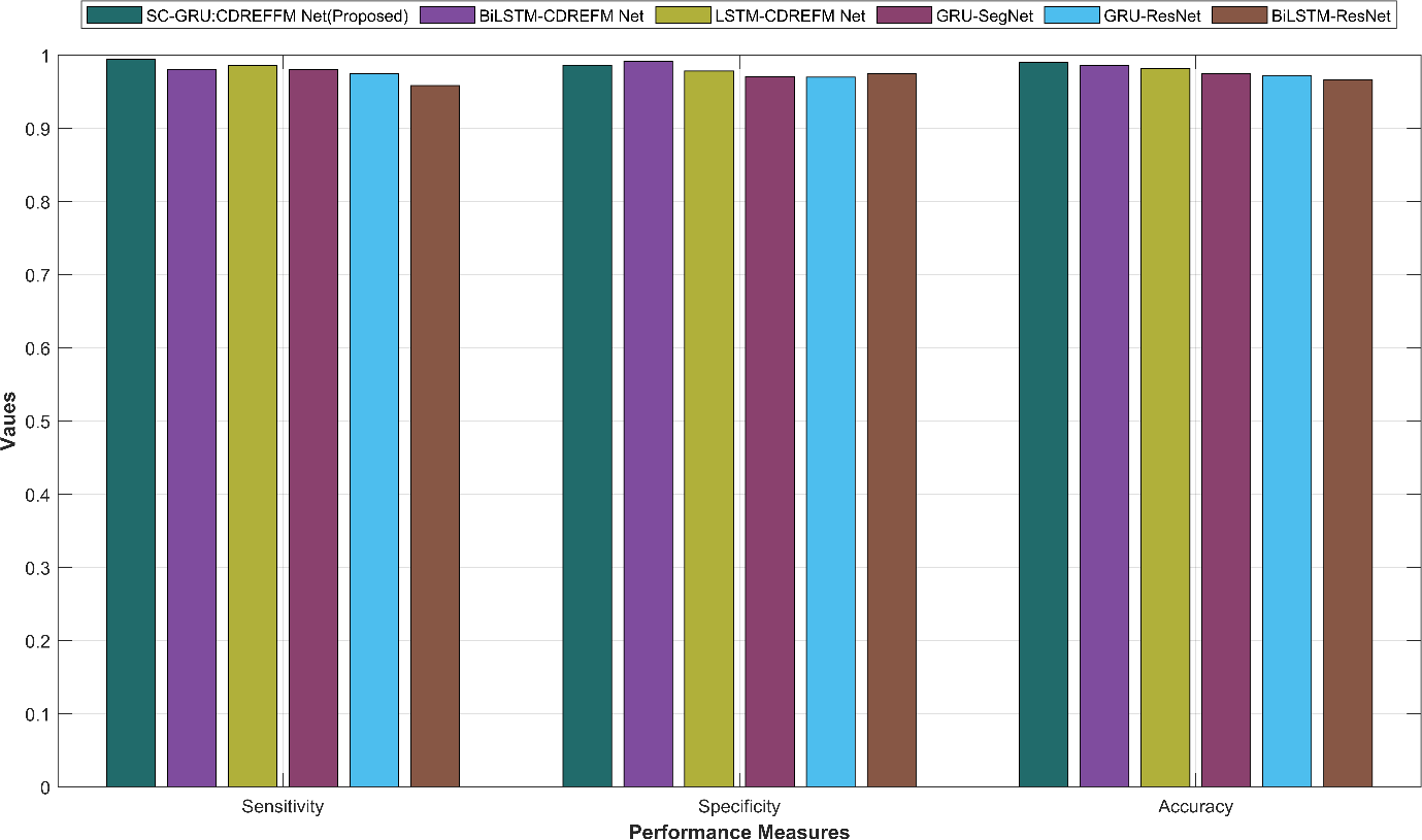
Figure 2: Graphical representation of the performance metrics Sensitivity, Specificity, and accuracy

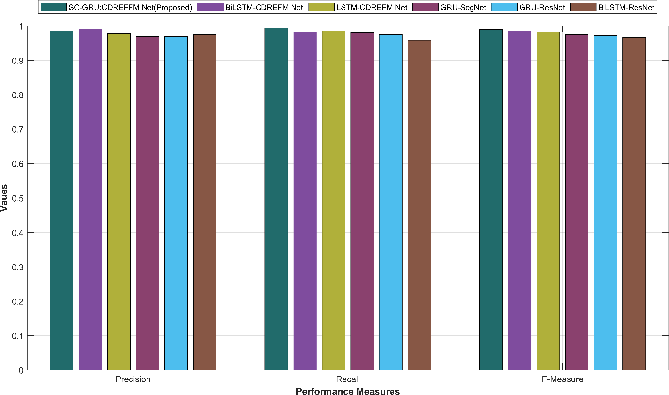
Figure 3: Graphical representation of the performance metrics precision, recall, and F-measure

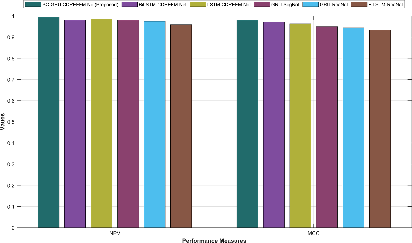
Figure 4: Graphical representation of the performance metrics NPV and MCC

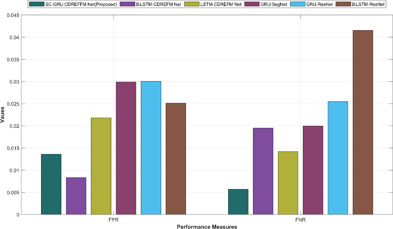
Figure 5: Graphical representation of the performance metrics FPR and FNR

(b)

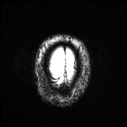
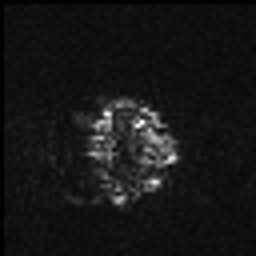
Figure 6: AD (a) MRI (b) PET

(b)

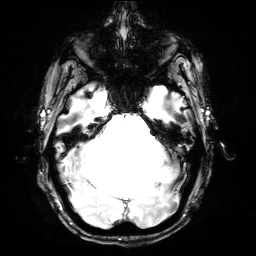
Figure 7: CN (a) MRI (b) PET

(b)

Figure 8: Fused images (a) MRI (b) PET

(b)

Figure 9: Pre-processed images (a) MRI (b) PET

(b)

Figure 10: Segmented images (a) MRI (b) PET

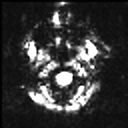
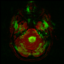
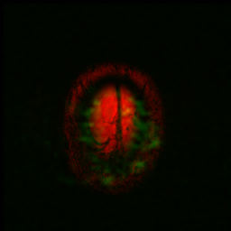
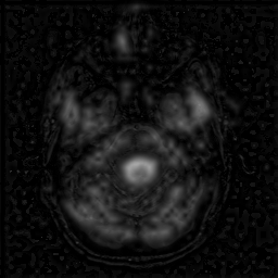
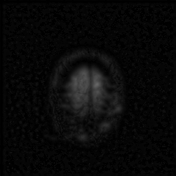
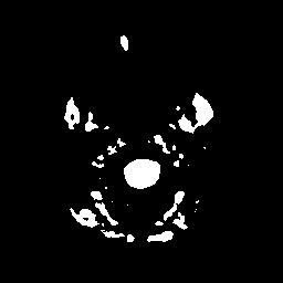
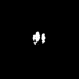
Figure 6 displays AD images, featuring (a) MRI and (b) PET modalities. In Figure 7, CN images are presented with (a) MRI and (b) PET modalities. Figure 8 exhibits fused images, combining (a) MRI and (b) PET modalities for enhanced analysis. Figure 9 demonstrates pre-processed images for both (a) MRI and (b) PET modalities. Lastly, Figure 10 showcases segmented images from (a) MRI and (b) PET modalities, illustrating the outcomes of the segmentation process.

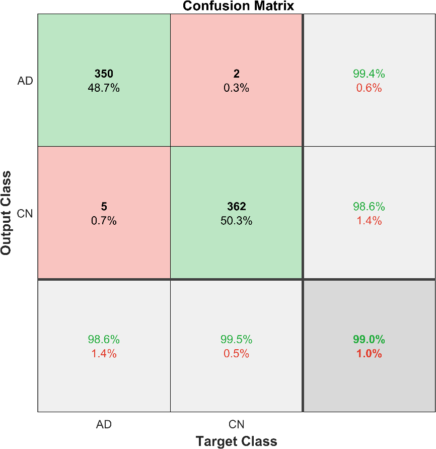
Figure 11: Confusion Matrix

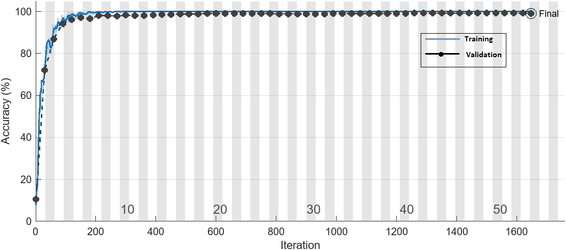
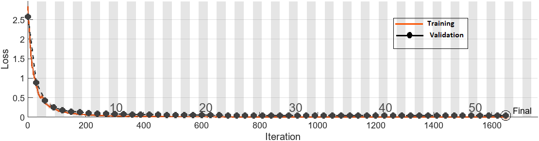
The confusion matrix in Figure 11 shows the model’s correct and incorrect predictions. Figure 12 presents the validation accuracy and loss curves used to examine generalisation to unseen data.

(a)

(b)

Figure 12: Validation (a) accuracy and (b) loss

Conclusion

AD is a progressive neurological disorder characterised by memory loss and cognitive deterioration. Advances in biomedicine have made CAD a useful tool for early and precise detection. This multimodal strategy included MRI, CT and PET data to improve stability, progression detection and diagnostic robustness. The CAD process began with image preparation because the collected images often contained noise that could hinder segmentation and classification. Geometric transformations, image augmentation, noise reduction and grayscale conversion were applied alongside LEWHE, ASSO and guided image denoising. These methods refined the data for segmentation and classification. The study introduced CDREFM_Net, which used the CICSC algorithm for semantic segmentation and high-level feature learning. RFF and different kernel sizes improved feature learning through entropy and dilation. GRU captured sequential dependencies for classification. Python was used to implement the proposed model.

References

Zhang, J., Zheng, B., Gao, A., Feng, X., Liang, D. and Long, X., 2021. A 3D densely connected convolution neural network with connection-wise attention mechanism for Alzheimer’s disease classification. Magnetic Resonance Imaging, 78, pp.119-126.

Liu, M., Li, F., Yan, H., Wang, K., Ma, Y., Shen, L., Xu, M. and Alzheimer’s Disease Neuroimaging Initiative, 2020. A multi-model deep convolutional neural network for automatic hippocampus segmentation and classification in Alzheimer’s disease. Neuroimage, 208, p.116459.

Liu, L., Liu, S., Zhang, L., To, X.V., Nasrallah, F. and Chandra, S.S., 2023. Cascaded multi-modal mixing transformers for alzheimer’s disease classification with incomplete data. NeuroImage, 277, p.120267.

AbdulAzeem, Y., Bahgat, W.M. and Badawy, M., 2021. A CNN based framework for classification of Alzheimer’s disease. Neural Computing and Applications, 33, pp.10415-10428.

Jain, R., Jain, N., Aggarwal, A. and Hemanth, D.J., 2019. Convolutional neural network-based Alzheimer’s disease classification from magnetic resonance brain images. Cognitive Systems Research, 57, pp.147-159.

Helaly, H.A., Badawy, M. and Haikal, A.Y., 2021. Deep learning approach for early detection of Alzheimer’s disease. Cognitive computation, pp.1-17.

Ramzan, F., Khan, M.U.G., Rehmat, A., Iqbal, S., Saba, T., Rehman, A. and Mehmood, Z., 2020. A deep learning approach for automated diagnosis and multi-class classification of Alzheimer’s disease stages using resting-state fMRI and residual neural networks. Journal of medical systems, 44, pp.1-16.

Basheera, S. and Ram, M.S.S., 2020. A novel CNN based Alzheimer’s disease classification using hybrid enhanced ICA segmented gray matter of MRI. Computerized Medical Imaging and Graphics, 81, p.101713.

Maqsood, M., Nazir, F., Khan, U., Aadil, F., Jamal, H., Mehmood, I. and Song, O.Y., 2019. Transfer learning assisted classification and detection of Alzheimer’s disease stages using 3D MRI scans. Sensors, 19(11), p.2645.

Hazarika, R.A., Abraham, A., Kandar, D. and Maji, A.K., 2021. An improved LeNet-deep neural network model for Alzheimer’s disease classification using brain magnetic resonance images. IEEE Access, 9, pp.161194-161207.

An, N., Ding, H., Yang, J., Au, R. and Ang, T.F., 2020. Deep ensemble learning for Alzheimer’s disease classification. Journal of biomedical informatics, 105, p.103411.

Shao, W., Peng, Y., Zu, C., Wang, M., Zhang, D. and Alzheimer’s Disease Neuroimaging Initiative, 2020. Hypergraph based multi-task feature selection for multimodal classification of Alzheimer’s disease. Computerized Medical Imaging and Graphics, 80, p.101663.

Janghel, R.R. and Rathore, Y.K., 2021. Deep convolution neural network based system for early diagnosis of Alzheimer’s disease. Irbm, 42(4), pp.258-267.

Basheera, S. and Ram, M.S.S., 2019. Convolution neural network–based Alzheimer’s disease classification using hybrid enhanced independent component analysis based segmented gray matter of T2 weighted magnetic resonance imaging with clinical valuation. Alzheimer’s & Dementia: Translational Research & Clinical Interventions, 5, pp.974-986.

Basaia, S., Agosta, F., Wagner, L., Canu, E., Magnani, G., Santangelo, R., Filippi, M. and Alzheimer’s Disease Neuroimaging Initiative, 2019. Automated classification of Alzheimer’s disease and mild cognitive impairment using a single MRI and deep neural networks. NeuroImage: Clinical, 21, p.101645.

G. Palacios-Navarro, J. Buele, S. Gimeno Jarque and A. Bronchal García, “Cognitive Decline Detection for Alzheimer’s Disease Patients Through an Activity of Daily Living (ADL),” in IEEE Transactions on Neural Systems and Rehabilitation Engineering, vol. 30, pp. 2225-2232, 2022, doi: 10.1109/TNSRE.2022.3196435.

K. Li et al., “Feature Extraction and Identification of Alzheimer’s Disease based on Latent Factor of Multi-Channel EEG,” in IEEE Transactions on Neural Systems and Rehabilitation Engineering, vol. 29, pp. 1557-1567, 2021, doi: 10.1109/TNSRE.2021.3101240.

N. Mccombe et al., “Alzheimer’s Disease Assessments Optimized for Diagnostic Accuracy and Administration Time,” in IEEE Journal of Translational Engineering in Health and Medicine, vol. 10, pp. 1-9, 2022, Art no. 4900809, doi: 10.1109/JTEHM.2022.3164806.

A. Basher, B. C. Kim, K. H. Lee and H. Y. Jung, “Volumetric Feature-Based Alzheimer’s Disease Diagnosis From sMRI Data Using a Convolutional Neural Network and a Deep Neural Network,” in IEEE Access, vol. 9, pp. 29870-29882, 2021, doi: 10.1109/ACCESS.2021.3059658.

X. Gao, F. Shi, D. Shen and M. Liu, “Task-Induced Pyramid and Attention GAN for Multimodal Brain Image Imputation and Classification in Alzheimer’s Disease,” in IEEE Journal of Biomedical and Health Informatics, vol. 26, no. 1, pp. 36-43, Jan. 2022, doi: 10.1109/JBHI.2021.3097721.

W. Liu, Q. Dong, S. Sun, J. Shen, K. Qian and B. Hu, “Risk Prediction of Alzheimer’s Disease Conversion in Mild Cognitive Impaired Population Based on Brain Age Estimation,” in IEEE Transactions on Neural Systems and Rehabilitation Engineering, vol. 31, pp. 2468-2476, 2023, doi: 10.1109/TNSRE.2023.3247590.

Y. Zhao, B. Ma, P. Jiang, D. Zeng, X. Wang and S. Li, “Prediction of Alzheimer’s Disease Progression with Multi-Information Generative Adversarial Network,” in IEEE Journal of Biomedical and Health Informatics, vol. 25, no. 3, pp. 711-719, March 2021, doi: 10.1109/JBHI.2020.3006925.

L. Brand, K. Nichols, H. Wang, L. Shen and H. Huang, “Joint Multi-Modal Longitudinal Regression and Classification for Alzheimer’s Disease Prediction,” in IEEE Transactions on Medical Imaging, vol. 39, no. 6, pp. 1845-1855, June 2020, doi: 10.1109/TMI.2019.2958943.

M. Ashtari-Majlan, A. Seifi and M. M. Dehshibi, “A Multi-Stream Convolutional Neural Network for Classification of Progressive MCI in Alzheimer’s Disease Using Structural MRI Images,” in IEEE Journal of Biomedical and Health Informatics, vol. 26, no. 8, pp. 3918-3926, Aug. 2022, doi: 10.1109/JBHI.2022.3155705.

S. Ahmed et al., “Ensembles of Patch-Based Classifiers for Diagnosis of Alzheimer Diseases,” in IEEE Access, vol. 7, pp. 73373-73383, 2019, doi: 10.1109/ACCESS.2019.2920011.

van Oostveen, W.M. and de Lange, E.C., 2021. Imaging techniques in Alzheimer’s disease: a review of applications in early diagnosis and longitudinal monitoring. International journal of molecular sciences, 22(4), p.2110.

Tamanini, I., Pinheiro, P.R. and Pinheiro, M.C.D., 2010. The choice of neuropathological questionnaires to diagnose the alzheimer’s disease based on verbal decision analysis methods. In Information Computing and Applications: First International Conference, ICICA 2010, Tangshan, China, October 15-18, 2010. Proceedings 1 (pp. 549-556). Springer Berlin Heidelberg.

Editorial Staff

Academic Master Education Team is a group of academic editors and subject specialists responsible for producing structured, research-backed essays across multiple disciplines. Each article is developed following Academic Master’s Editorial Policy and supported by credible academic references. The team ensures clarity, citation accuracy, and adherence to ethical academic writing standards

Content reviewed under Academic Master Editorial Policy.

• Editorial Staff

  Grid-Connected Solar PV Systems and Power Quality Review
• Editorial Staff

  Predicting Cardiovascular Diseases with PCA and Artificial Neural Networks
• Editorial Staff

  Maternal and Neonatal Outcomes Following Water Birth Systematic Review and Meta-Analysis
• Editorial Staff

  Electrospun Polymeric Nanofibers for Biomedical Applications