Intelligent Routing of Delay-Tolerant Networks with Hybrid Whale-Teach Optimisation

Abstract

Delay-tolerant networks (DTNs) lack permanent connections between nodes. When a node receives a message from one of its contacts, it faces the challenge of store-carry-forward (SCF) routing. This study presents an approach to intelligent routing in DTNs. It begins by gathering information about network topology, historical performance metrics and communication patterns from network nodes. The second stage establishes a framework centred on five objectives for optimal path identification. These objectives prioritise maximising the delivery ratio, minimising message latency, reducing the overhead ratio, optimising social network characteristics and balancing these goals to improve routing efficiency. The final stage introduces Hybrid Whale-Teach Optimisation (HWTO), which combines the Whale Optimisation Algorithm (WOA) and Teaching-Learning-Based Optimisation (TLBO) to select routes according to the specified objectives. The approach offers potential applications in challenging communication environments and aims to improve the reliability and performance of message routing in DTNs.

Keywords: Delay-tolerant networks, store-carry-forward, Five-Fold Objectives, Hybrid Whale-Teach Optimisation, and message routing.

Introduction

Paths between a source and a destination may not always be available, making DTNs suitable for sparse networks. SCF procedures allow a node to retain data until it encounters a neighbour that can forward it. Other networks can also help bridge communication gaps. As network connectivity increases, cooperation can improve message delivery. Unmanned aerial vehicles (UAVs) are frequently used as auxiliary relays in DTNs [1,2,3]. Because DTN nodes are mobile and intermittently connected, reliable, continuous end-to-end connections between sources and destinations cannot be assumed. These conditions can produce substantial delivery delays. DTNs are designed to operate over sporadic connections, with SCF patterns forming the foundation of routing [4,5,6].

By adopting this method, DTNs make it possible to communicate in sparse regions without end-to-end connection. In a DTN, a node keeps the message it wishes to transmit and circulates with it until it encounters another node [7,8], at which time it passes a copy of the message. Until either the message’s time to live (TTL) expires or it reaches the target node, the receiving node will continue acting in the same way. Changing messages is the name of this procedure. The wait time for a link to establish, which might take some time, has an impact on the asymmetric data rate. Interplanetary communication was the inaugural use of DTNs, when opportunistic contacts and a store-carry-and-forward technique were implemented [9,10]. However, DTN communication designs may also be employed in applications for rural and undeveloped areas. Multiple copies of the same message will be individually routed around the network. This method will quicken data transmission and reduce typical delays. This method has the problem of wasting network traffic and node storage [11,12,13].

A node with a communication interface and a buffer can transmit or forward messages in a DTN. A major limitation of these models is the energy consumed during transmission, storage and reception. Mobile nodes may be unable to reach an electrical outlet when their batteries run low [14,15]. A routing mechanism must therefore achieve a high delivery probability while limiting energy consumption and buffer use. This study compares routing performance using delivery ratio, delay, social network parameters, overhead ratio and the trade-offs involved in optimal path identification. The main contributions are as follows.

In order to enhance the WOA’s encircling behaviour, the TLBO algorithm’s teaching factor can be included. This is a crucial step in improving the performance of these algorithms, especially when used with DTNs. The efficiency with which nearby nodes may be found inside a DTN model is anticipated to be improved by this merging of the two algorithms.

By changing the whale’s spiral position using the learner phase of the TLBO algorithm, it is feasible to prevent the algorithm from being stuck in local optima. This approach, which utilises both the spiral movement and the learner phase of TLBO, aids in the pursuit of the optimal solutions.

This paper is organised as follows. Section 2 reviews recent DTN research. Section 3 describes the proposed methodology. Section 4 presents the MATLAB results and compares them with existing techniques. Section 5 concludes the paper.

Literature Review

In this section, the recent existing papers related to the DTN used for optimal path selection are discussed with their drawbacks.

In 2021, Wu et al. [16] described a social-circle formation technique based on node clustering in DTNs. They proposed the SC-SS spray approach, which uses social circles and differences in node-forwarding capability to improve spray-and-wait routing. SC-SS selects the next hop according to social connections between nodes during the spray stage. To improve performance further, the authors developed the adaptive SC-AMSW routing method. Rather than fixing the initial number of copies, SC-AMSW determines the number of duplicate messages from the delivery likelihood during the waiting interval and sprays copies adaptively.

In 2021, Wu et al. [17] presented Fuzzy Logic-based Double Q-Learning Routing (FDQLR), which combines the DQL algorithm with fuzzy logic to identify routes. Its dynamic reward system uses fuzzy logic to analyse contact intervals, node activity and movement speed. The authors also recommended hot-zone and message-dropping mechanisms to improve message forwarding and buffer handling.

In 2020, McGeehan et al. [18] introduced ChitChat for social-context-based message delivery in sparse DTNs. ChitChat is a hybrid geographic and data-centric routing system that learns multi-hop pathways and interprets locations through user route planning and social connections. It uses each user’s social or mission interests to support routing when connections are scarce.

In 2021, Chinnasamy et al. [19] introduced multi-objective throwbox deployment for DTNs in Internet of Things (IoT) environments. DTN models can address intermittent connectivity in IoT architectures. In a throwbox-assisted DTN-IoT setting, the study identifies deployment locations by improving delivery ratios and throwbox accessibility while reducing average delay.

In 2020, Bakiras et al. [20] examined secure and anonymous communication over DTNs. Their message-forwarding mechanism uses random walks to convey messages from source to destination without revealing intermediary nodes along the route. They recommended two encryption methods: a public-key approach for short messages such as SMS, and a hybrid public-key and symmetric-key approach for larger multimedia messages, including photographs and videos.

In 2020, Juyal et al. [21] proposed dynamic trusted routing for high-density DTNs. Their threshold-based approach cooperates with conventional routing protocols when the network becomes sparse. The first phase selects trustworthy nodes using a logistic activation function. The second creates trusted clusters using a threshold and removes non-cooperative nodes. The third uses a dynamic routing mechanism to forward messages.

In 2021, Rehman et al. [22] recommended a message-dropping policy to improve buffer management in DTNs. Spontaneous Size Drop (SS-Drop) first calculates the difference between the incoming message size and the available buffer space, then determines how much data to discard. The authors assessed the policy using shortest-path map-based mobility models and Epidemic routing. Under the most effective map-based model, SS-Drop outperformed Drop Front (DF), Drop Oldest (DOA) and Drop Largest (DLA) in delivery probability and overhead ratio.

In 2022, Chatterjee et al. [23] examined routing-attack detection in DTNs. Their study described malicious activities, their network effects and the difficulties encountered during message transmission. It also considered the damaging behaviour of rogue nodes. Protecting DTNs from unauthorised access, resource misuse and data alteration remains a challenging area of network-security research.

In 2022, Velusamy and Lent [24] applied a spiking neural network to DTN routing. Satellite missions require routing strategies that balance high throughput with low latency. The study modified Kleinrock’s power metric to reduce delay and packet loss and evaluated its performance. For NASA’s High Rate Delay Tolerant Networking (HDTN) project, the authors used a cognitive space-routing strategy based on a reinforcement-learning spiking neural network.

In 2021, Ayub and Rashid [25] introduced an energy-efficient routing protocol based on inactive-node detection in DTNs. The technique uses node mobility to identify inactive nodes. A buffer-management system also detects and ignores messages addressed to inactive nodes. Real-time mobility models were used to compare the protocols in terms of broadcasts, dropped messages, deliveries and average hop count.

Problem Statement

In the domain of DTNs, a variety of inventive routing protocols and buffer management techniques have surfaced, each presenting distinctive resolutions to the obstacles of intermittent connectivity and node mobility. Nonetheless, a noteworthy predicament is the absence of a consolidated assessment framework, thereby rendering it arduous to comprehensively compare these approaches. Additionally, matters such as scalability, security, and energy efficiency persist as focal points of concern. The assurance of security and privacy in data transmission is of utmost importance, necessitating robust measures against various forms of attacks. Particularly in environments with limited resources, it is crucial to optimise buffer management policies. Additionally, it is important to investigate how to integrate DTNs with cutting-edge technologies like satellite communication and the Internet of Things. Detecting inactive nodes and routing that takes mobility into account are other issues that must be addressed for a network to operate effectively. As a result, even though DTN research has made significant strides, there is still a pressing need for effective path selection techniques to guarantee timely and accurate message delivery in these complex and dynamic network environments.

Proposed Methodology

DTNs are a special class of networks where it is impossible to assume constant network connectivity because the nodes involved are mobile. The lack of end-to-end and continuous connection pathways in DTNs always causes message delivery delays. This paper presents an overview of DTNs with a focus on how they function in circumstances with sporadic connections between nodes. The idea of SCF routing, in which nodes store messages received from contacts in their buffer and transport them opportunistically when coming into touch with other nodes, is essential to how they work. This strategy, however, faces a significant obstacle known as “optimal routing.” This research presents a comprehensive strategy to optimize intelligent routing in DTNs through a five-fold objective optimization framework with a hybrid optimization approach that combines WOA and TLBO. Our methodology aims to enhance the efficiency of data routing in DTNs. This section outlines a detailed step-by-step workflow that encompasses advanced concepts, ultimately leading to more effective and efficient data routing in challenging network scenarios. The diagrammatic representation of optimal path selection in DTN is shown in figure 1.

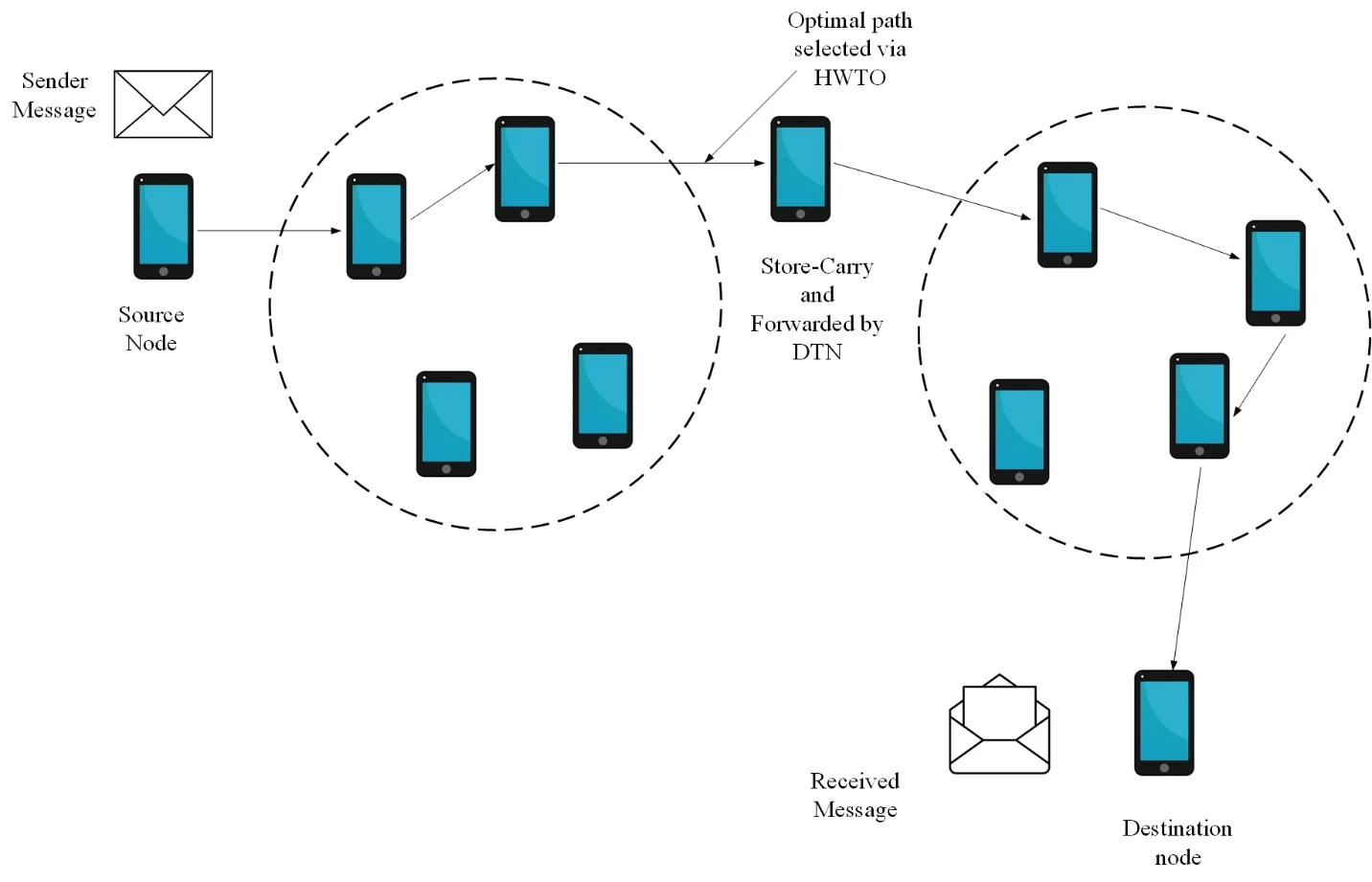
Figure 1: Message transmission Via nodes with DTN

Data Collection

The nodes in this study are homogeneous in hardware and initial energy. Their speed, mobility model and neural-network information may differ. Each node can execute the algorithm independently and can generate, send or receive messages. Depending on the message, a node may take one of four roles:

Source node

Secondary destination

CBTD

Destination

Source node

A source node carries a message, interacts with other nodes, executes the proposed algorithm and decides whether to forward the message.

Secondary destination

A secondary destination lies outside the source node’s communication range and offers a favourable opportunity to carry the message to its destination. Once this node is identified, the source attempts to route the message to it before it encounters the destination. The source recognises at most one unvisited node as the secondary destination; it may identify none.

CBTD

CBTD stands for Contact node with Better circumstances to Take the message to the Destination node. It is a contacted node that is better positioned to deliver the message, either by reaching the destination sooner or by reaching a suitable secondary destination sooner. The source recognises at most one contacted node as its CBTD and may identify none.

Destination

The message needs to go to this node. It’s difficult to route in DTN. Because of node mobility, future relationships between nodes are unclear and confusing. Furthermore, there aren’t always direct, continuous connections between source and destination nodes. Considering that the broadcast range is often greater than the distance between the source and destination nodes, the source node cannot always directly interact with the destination node. For the routing operation, DTNs employ a SCF method. When a node in a SCF mechanism gets a message from one of its contacts, it stores it in its buffer and broadcasts it until it connects with another contact node (CBTD) that has more favourable conditions to deliver the message to the destination node. For routing to be effective, messages must be forwarded to CBTD, and this action plays a crucial part in routing effectiveness. In addition, CBTDs will enable communications to get to their destination more quickly.

In this study, routing is carried out by selecting the appropriate nodes. For routing, no node attempts to obstruct it. In terms of routing, the source node transmits the message to CBTD after recognising it. The source node holds onto the data in its buffer in the event that none of the contacted nodes recognise CBTD, hoping that it will eventually reach the destination by itself or recognise CBTD. The route in a DTN that maximises the possibility of successful message delivery while minimising latency and overhead is known as the optimum path. Finding the best path involves choosing contact nodes with favourable circumstances.

Five-Fold Objectives based optimal path identification

Due to the sporadic connection and dynamic nature of DTNs, finding the optimal path through a network can be challenging. Consider a set of five goals that balance diverse aspects in order to choose the best course of action. These goals aid in choosing a course of action that minimises delay, overhead, and resource consumption while increasing the possibility of effective message delivery. The several objectives, including delivery ratio, overhead ratio, delay, social network factors, and balancing trade-offs are also considered.

i) Maximize Delivery Ratio

The percentage of messages that successfully arrive at their intended locations inside the DTN is known as the delivery ratio. The basic goal of DTNs is to maximise the delivery ratio. It makes sure that messages are efficiently sent over the network even in areas with poor connection. DTN routing protocols and techniques should be created to make effective use of network resources, optimise message replication, and take advantage of opportunistic communication possibilities when nodes come into contact in order to maximise delivery ratio.

The delivery ratio is a statistic employed in networking to assess how well data packets are delivered from a source to a destination. The following Eq. (1) is used to compute it, which is frequently stated as a ratio or percentage:

        (1)

Where stands for the number of delivered packets, denotes the number of packets sent from the source node. The delivery ratio offers perceptions into the dependability and effectiveness of data transmission in a network. A network with a greater delivery ratio is considered to be more dependable, whereas one with a lower delivery ratio may imply that a sizable fraction of transmitted packets did not arrive at their intended destination.

ii) Minimize Delay

The amount of time it takes for messages to travel across the network from their source node to their destination node is expressed as delay in DTNs. In applications like real-time data collecting or emergency response where quick message transmission is critical, minimising latency is essential. Message queuing and waiting times are reduced, routing decisions are optimised, and priority forwarding is given to nodes that are closer to the destination as part of DTN routing protocols’ efforts to minimise latency.

DTNs differ from standard networks in that they have occasional connectivity and store-and-forward routing, in which messages are forwarded as soon as a network connection is established. A DTN’s latency may be visualised as the sum of a number of factors:

Transmit Delay (): This is the amount of time needed for a message to go from the source node to the first relay or storage node. It depends on how quickly the communication channel transmits data.

Propagation Delay (): This is the amount of time it takes for a message to spread over the network from one node to another. It is influenced by the medium’s propagation speed and the separation between nodes.

Queueing Delay (): Until they can be transmitted to the following hop, messages in DTNs are frequently kept in buffers at the nodes. The amount of time a message waits in these buffers before being sent is called the queuing delay.

Relay Delay (): This is the lag time that results from messages being held at intermediate relay nodes prior to being delivered to their final destination. Depending on the duration that a message is kept on buffer at each relay node.

These elements are added to represent overall DTN latency in Equation (2):

      (2)

This equation captures the special difficulties and features of DTNs, where messages may be delayed as they move across the network via opportunistic transmission and nodes may become disconnected for long periods of time. In order to provide effective data transmission, DTNs must manage and minimise latency, especially in situations like distant or sparse communication settings, disaster recovery, and interplanetary communication.

iii) Minimize Overhead Ratio

The term “overhead” in DTNs refers to the extra resource needs incurred during the transmission of messages, including bandwidth, power, and storage space. In resource-constrained settings or when energy is a crucial issue, minimising overhead is crucial for network resource conservation. DTN protocols should carefully control message duplication, routing choices, and message trimming to ensure that excessive resource usage is reduced.

The overhead ratio is a statistic used in DTNs to assess the amount of extra data added to the network in addition to the real user data that is being carried. It is frequently used in DTNs, where effective network resource utilisation is essential owing to patchy connection and constrained bandwidth, to assess the effectiveness of routing and communication protocols. The following Eq. (3) may be used to compute the overhead ratio and can be used to represent it as a ratio or percentage:

      (3)

The term “overhead data size” refers to the amount of data that is introduced into the network for the purpose of routing and control, including acknowledgments, control messages, routing headers, and any other data that is not original user data. User data size refers to the volume of user-generated data that is actually sent across a network.

The overhead ratio sheds light on the effectiveness of the network’s management and routing processes in relation to the data that actually belongs to the users. In general, a lower overhead ratio is preferred since it means that less of the network’s resources are being utilised for overhead activities, freeing up more bandwidth for user data transfer. In situations when network resources are limited or expensive to maintain, efficient routing and communication protocols seek to reduce the overhead ratio in DTNs to guarantee that precious resources are used wisely.

iv) Optimize Social Network Parameters

Optimizing social network parameters, such as trust and distance, can indeed enhance routing efficiency in DTNs. These parameters are crucial for making informed routing decisions in situations where network connectivity is intermittent and nodes rely on social characteristics to forward messages.

Social strength

A node’s social strength depends on the number of its social connections. An intermediate node B with stronger social connections is more likely to encounter other nodes and forward additional message copies. This can reduce delay at the cost of a higher overhead ratio.

Friendship

People who share interests, behave similarly and meet frequently are likely to form strong friendships. The vehicular DTN (VDTN) concept of friendship follows this principle, using declared shared interests to determine the relationship between two nodes.

Selfishness

A VDTN node’s selfishness may be identified by how it treats its social relationships and itself. A selfish node could ignore other nodes’ messages in favour of repeating its own or its friends’ messages. Selfishness, in contrast to all the other network metrics stated above, is viewed as a bad social trait. Selfish activity on the part of a node enhances the delivery rate of his social ties at the expense of the performance of other nodes. For instance, source node A would only benefit from sending the message to self-centred intermediary node B if they were socially connected. The social connection may consist of their friendship or community.

Trust

A node’s confidence in a wireless network may be expressed by its reliability, utility, availability, quality of services, and other equivalent characteristics. For the sake of our work, trust specifically refers to the degree of belief that the source node places in the intermediary node regarding the message’s delivery based on earlier behavioural observation. It is the total amount of messages that the intermediate node has successfully transmitted during the course of its existence, in terms of mathematics. The trust level of a node is defined as a real value in [0, 1], with 1 denoting total trust, 0.5 denoting ignorance, and 0 denoting complete mistrust. At time , node evaluated node ‘s trust value, indicated in Eq. (4), is derived by a weighted average of healthiness, unselfishness, connection, and energy as follows:

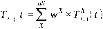          (4)

Where stands for a trust property that has been studied ( can be healthiness, unselfishness, connectedness, or energy), Eq. (4) represents the trust that node has for node , and is the weight attached to trust property with a total of one.

v) Balance Trade-offs

Finding the best methods that balance the goals of maximising delivery ratio, minimising latency, and minimising overhead while optimising social network characteristics is necessary for balancing trade-offs in DTNs. Due to the inherent difficulties of sporadic connection and resource limitations, DTNs sometimes need trade-offs between these objectives. Designing routing protocols and techniques that dynamically adjust to network conditions and prioritise goals based on the particular application and environment is necessary to achieve a balance. While trade-offs in DTNs are typically discussed qualitatively, they can also be represented mathematically using equations or formulas.

Delivery Delay vs. Message Overhead

One common trade-off in DTNs is between minimizing delivery delay and controlling message overhead. Increasing the number of copies of a message (to reduce delay) also increases message overhead, shown in Eq. (5),

        (5)

Delivery Probability vs. Message Overhead

Balancing the probability of successful message delivery and message overhead is essential in DTNs. Increasing message copies can improve delivery probability but at the cost of higher overhead, which is denoted in Eq. (6) as,

      (6)

Delivery Probability vs. Relaying Density

Trade-off Equation: Increasing the density of relaying nodes in the network can improve message delivery probability, but it may also lead to higher resource utilization and energy consumption. The relation between delivery probability and relaying density is shown in Eq. (7),

      (7)

Energy Efficiency vs. Data Rate

Trade-off Equation: In energy-constrained DTN scenarios, there’s often a trade-off between maximizing energy efficiency and achieving a higher data transmission rate. Transmitting data at a higher rate may consume more energy per unit of data. The relation between Energy efficiency and data rate is given in Eq. (8) as,

        (8)

Node Mobility vs. Network Connectivity

Node mobility can affect network connectivity. Higher node mobility may lead to more frequent network partitions, but it can also enhance message dissemination opportunities. The relation between network connectivity and node mobility is given in Eq. (9) as,

      (9)

Delivery Ratio vs. Buffer Size

Trade-off Equation: Increasing the buffer size at nodes can improve the delivery ratio by storing more messages for future relaying opportunities. However, larger buffers may lead to resource wastage, which is shown in Eq. (10).

      (10)

The HWTO algorithm is introduced to solve these multi-objective problems and select an optimal path. It combines whale-inspired search behaviour with teaching-learning-based optimisation to address the competing routing objectives.

Hybrid Whale-Teach Optimization (HWTO)

Hybrid Whale-Teach Optimisation (HWTO) combines WOA and TLBO to identify an optimal path. WOA is inspired by the hunting behaviour of humpback whales, particularly bubble-net feeding. Whales descend to a depth of about 12 metres, encircle prey with spiral-shaped bubbles and move towards the surface. This behaviour provides the basis for the algorithm’s search and position-updating procedures.

Combining WOA with TLBO uses the strengths of both algorithms and may accelerate convergence in complex, high-dimensional optimisation problems. WOA supports exploration of the search space, while TLBO helps exploit promising locations. Their integration aims to balance the search for new solutions with refinement of existing ones. The mathematical model for HWTO is presented below.

Teaching factor-based prey encircling

Humpback whales are capable of finding and circling their prey when hunting. When the target prey or a site nearby it is where the best search agent is currently situated, the HWTO algorithm takes that into consideration, and other search agents will make an effort to move into a position that is closer to the best search agent. The following Eq. (11) and Eq. (12) represent this behaviour:

        (11)

        (12)

Where is the current iteration, represents the position vector of each agent, denotes the absolute value, represents the position vector of the best solution found thus far in iteration and denotes a multiplication operation. It is determined how to calculate the coefficient vectors and .

The basic WOA technique used for evaluating the factor , which has the value of 2 to 0. So, the value of is decreasing. When is set to decrease too rapidly, it can lead to premature convergence. This means that the algorithm may converge to a suboptimal solution before thoroughly exploring the search space. On the other hand, if decreases too slowly, it can slow down the convergence speed of the algorithm, making it inefficient. Therefore, the teaching factor from the TLBO algorithm is combined with WOA optimisation to evaluate the updated position of the whale.

          (13)

            (14)

Where is a random value in [0, 1] and is a teaching factor that determines how much the mean should be altered. A further heuristic step that is chosen at random with the same probability as the value of , which has two possible values of 1 or 2, can be

        (15)

Bubble-net attacking strategy

The Bubble-net strategy combines two strategies, and it may be mathematically expressed as follows:

Shrinking Encircling Mechanism

By lowering the value of in Eq. (15), this behaviour of whales can be mimicked. Also take note of how increase the fluctuation range. By using random values for in the range [-1,1], the updated position of a search agent may be determined anywhere between the agent’s starting position and the position of the best agent at the moment.

Learner updated Spiral Updating Position (SUP)

The following spiral Eq. (16) is developed between the location of the whale and its prey in order to mimic the helix-shaped motions of humpback whales:

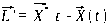          (16)

By enabling the search agents to more efficiently explore the search space, the learner equation can improve the algorithm’s capacity for exploration. This can lower the possibility of hitting local optima. For that, the learner phase of the TLBO is updated with the SUP phase of the WOA, which is represented in Eq. (17)

    (17)

Where represents the distance between the whale and its prey, determines the form of the logarithm, is a random variable in between [-1, 1]. Humpback whales move in a spiralling motion as well as a concentric circle motion. Iterations of the algorithm mimic picking either the spiral model movement or the diminishing encircling movement with a chance of 50%. That implies

  (18)

Where is a random variable and it ranges between [0,1].

Prey search phase

Most of the algorithms use random selection to search for the best solution. When using a bubble net, humpback whales hunt for prey at random since it is unknown where the ideal design will be. As opposed to ‘s exploitation phase, In this phase, assume that is a vector of random values greater than or equal to -1 but less than 1, in the range [-1,1]. This supposition gives the search agent the ability to go far from a reference whale. Instead of using the top search agent thus far, the position of the search agent will be modified according to a random selection of search agents. Following is a formulation of these two activities:

          (19)

          (20)

Where is a position vector chosen randomly.

A set of random solutions is used as the first step in the HWTO algorithm. The search agents adjust their location after each repetition in accordance with the previously mentioned justifications. Global optimizers include HWTO. The HWTO method transitions between exploration and exploitation swiftly thanks to adaptive alteration of the search vector A. Additionally, the HWTO only allows changes to two major internal parameters. Due to the whales’ position-updating system in Eq. (20), HWTO has a high degree of exploration capability. The emphasis is on high exploitation and convergence, which come from Eq. (17) and Eq. (12). These equations show how the HWTO method may provide high local optima avoidance and convergence speed throughout the course of an iteration. In algorithm 1, the HWTO algorithm’s pseudocode is displayed.

Results and Discussion

This section compares the proposed HWTO model with WOA, TLBO, Aquila Optimisation (AO) and Mayfly Optimisation (MFO). The algorithms are implemented in MATLAB. The source and destination nodes are stationary, while the remaining nodes move. Performance is evaluated across different node counts using delivery ratio, average delay, throughput, network lifetime and energy consumption. Table 1 lists the simulation parameters.

Table 1: Specifications of the simulation parameters

Delivery ratio

The delivery ratio compares the number of packets delivered to the destination with the number sent by the source. The objective is to deliver as many packets as possible. Table 2 reports the delivery ratios for different node counts.

Table 2: Comparison of the delivery ratio

Table 2 compares HWTO, WOA, TLBO, AO and MFO in networks containing 10–50 nodes. HWTO achieves delivery ratios between 0.93 and 0.97, with 0.97 at 10 nodes and 0.94 at 50 nodes. The ratios vary across the intermediate network sizes. TLBO records values between 0.77 and 0.92.

The Delivery Ratio values for the AO algorithm range from 0.87 to 0.80 for varied node counts. With values ranging from 0.84 to 0.64, the Delivery Ratio of the MFO technique considerably declines with network size. Figure 2 represents the various delivery ratios of the HWTO, WOA, TLBO, AO, and MFO.

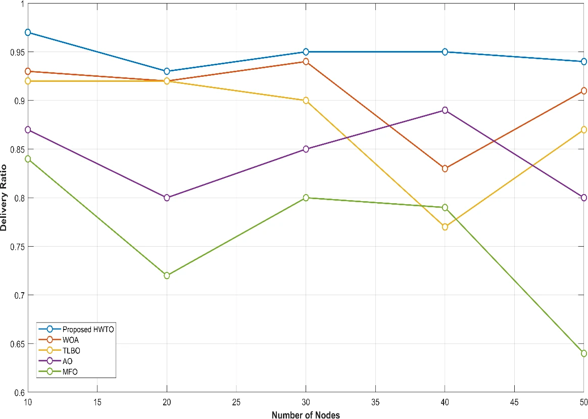
Figure 2: Graphical representation of the delivery ratio

Average delay

Average delay measures the time that delivered packets spend travelling through the network, including waiting at node buffers. Table 3 presents the average delay for each node count.

Table 3: Comparison of the average delay

HWTO’s average delay rises from 5 s with 10 nodes to 14.3 s with 50 nodes. WOA follows a similar pattern, increasing from 5.16 s to 14.87 s. These results show that latency increases as the simulated network grows.

The typical delay values for the TLBO algorithm range from 5.48s to 15.03s. Average delays for the AO technique range from 6.6s for 10 nodes to 16.6s for 50 nodes. This implies that although it functions excellently in smaller networks, its effectiveness declines as the network gets bigger. The MFO approach’s typical delays range from 7.92s to 17.07s seconds. This shows that the MFO strategy is less appropriate given the situation. The different average delay for the HWTO, WOA, TLBO, AO, and MFO are shown in Figure 3.

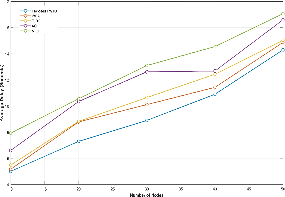
Figure 3: Graphical representation of the average delay

Throughput

Throughput measures the volume of information delivered per unit of time. Table 4 reports throughput in Kbps for each node count.

Table 4: Comparison of throughput

Between 437.6 Kbps and 357.89 Kbps, the “Proposed HWTO” algorithm regularly exhibits the highest throughput numbers. This implies that it successfully manages data transmission with high throughput performance even as the network scales. Although it gradually declines as the network capacity grows, the “WOA” algorithm displays competitive throughput performance. The range of “WOA”‘s throughput values is 420.99 Kbps to 345.6 Kbps. The “TLBO” algorithm’s throughput performance varies. It starts off with a pretty good throughput of 410.53 Kbps for 10 nodes, but as the network size grows, throughput decreases from 410.53 Kbps to 292.78 Kbps.

The “AO” algorithm regularly exhibits throughput values between 391.37 Kbps and 339.25 Kbps that are less than “WOA” and “Proposed HWTO.” In smaller networks, it keeps up a respectable performance, but as the network gets bigger, its throughput drops. Similar to this, the “MFO” algorithm displays throughput figures between 390.28 Kbps and 338.12 Kbps that are less than those of the top methods. Similar to “AO,” it sees a drop in throughput as the network size grows. The throughput for the HWTO, WOA, TLBO, AO, and MFO are shown in Figure 4.

Figure 4: Graphical comparison of throughput

Lifetime

It represents the period of time during which a node would be completely functional. One of the most popular ways to define a network’s lifespan is the moment at which the first node runs out of power while delivering a packet, as losing a node might cause the network to lose some functionality. Table 5 shows the lifetime when the node count is changed.

Table 5: Comparison of the lifetime

HWTO records the highest network lifetime at every tested node count. Its values range from 125.88 s to 287 s, falling initially and then increasing at 40 and 50 nodes. WOA records lifetimes between 116.43 s and 285.51 s. The results vary with network size rather than declining steadily.

As the network size increases, the Life Time is likewise shown to decrease via the TLBO method. A rather high Life Time of 278.78s for the first 10 nodes is followed by a decline to 111.65s for the following 50 nodes. The Life Time values of the AO algorithm are variable, starting at 277.34s for 10 nodes and peaking at 174.57s for 50 nodes. As the network grows, its Life Time goes through both ups and downs. The MFO method similarly shows a range of Life Time values, from 257.94s to 168.39s. Similar to AO, it fluctuates in Life Time as the network size grows. The lifetime of the nodes for the discussed techniques are shown in figure 5.

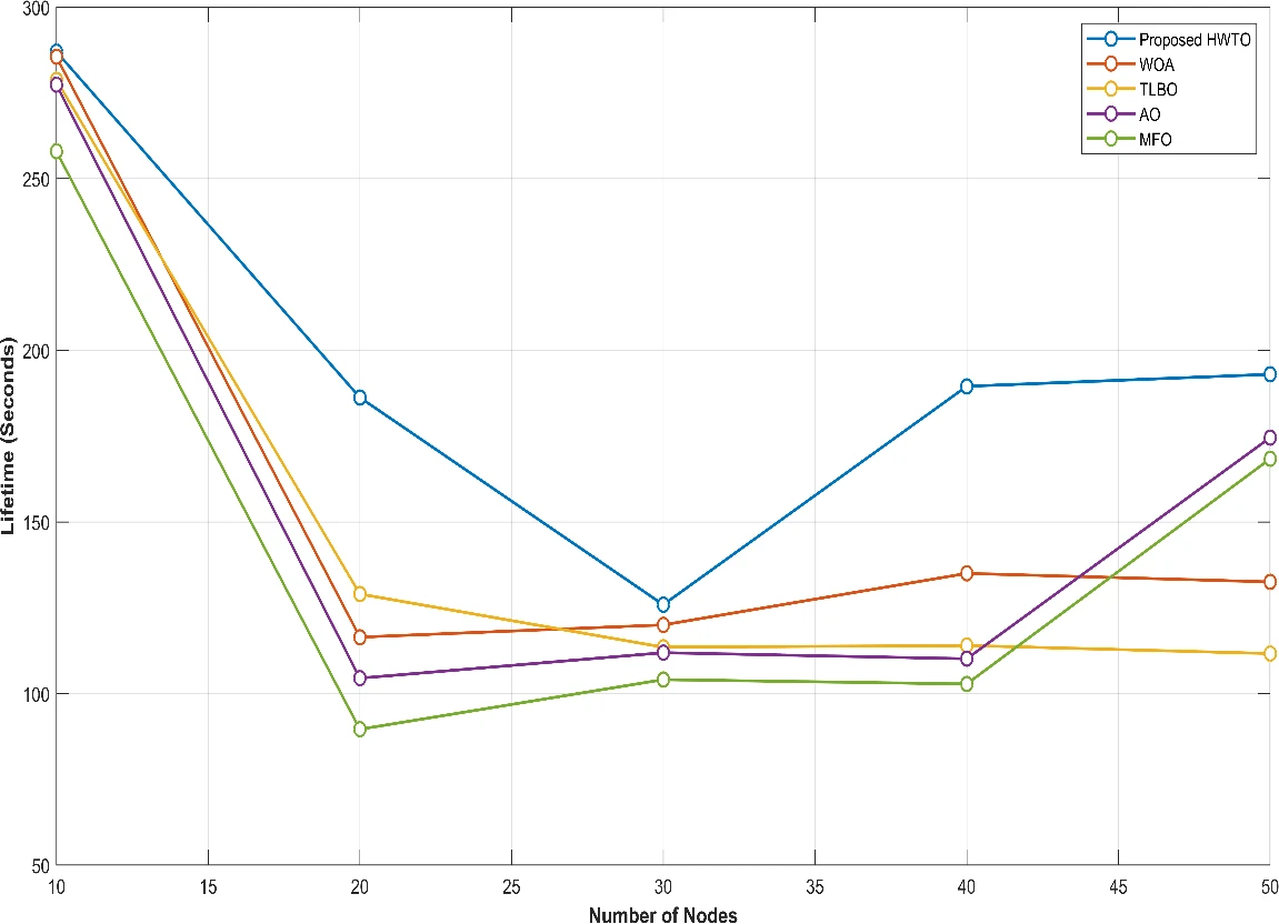
Figure 5: Graphical comparison of lifetime

Energy

Energy determines the total energy used by the entire network based on the energy used by each node while transmitting packets. Table 6 provides the total energy of the network as a function of the node count.

Table 6: Comparison of the energy

For all network sizes, the “Proposed HWTO” algorithm consistently shows the lowest energy usage numbers. With 10 nodes, it starts at 85.6 J and rapidly drops to 22.9 J with 50 nodes. This implies that even when the network goes up, the “Proposed HWTO” algorithm remains the most energy-efficient of the algorithms taken into account. Although reasonably stable across various network sizes, the “WOA” algorithm displays energy consumption numbers that are often greater than “Proposed HWTO”. Between 88.45 J and 38.36 J are the “WOA” values.

TLBO’s energy consumption decreases from 108.09 J with 10 nodes to 48.07 J with 50 nodes. AO records 114.66 J at 10 nodes and 58.67 J at 50 nodes, with variation between the tested sizes. MFO records values from 132.23 J to 53.88 J, ending at 69.35 J for 50 nodes. Figure 6 compares total network energy consumption across the algorithms.

Figure 6: Graphical comparison of the energy

Conclusion

In conclusion, this paper explores the complex issues DTNs encounter when network connectivity between nodes is sporadic or non-existent. The research emphasises a complete approach to intelligent routing within DTNs in order to address the critical issue of SCF routing. The study emphasises the value of assembling key data up front, including details on the network topology, historical performance indicators, and communication patterns between DTN nodes. This fundamental information forms the basis of an innovative paradigm for improving path identification within DTNs that is based on fivefold objectives.

These five-fold objectives place a high priority on important factors including optimising social network features, maximising message delivery ratio, minimising message delay, lowering overhead ratio, and striking a balance between these goals. This all-encompassing strategy aims to improve the efficacy and efficiency of message routing in DTNs. The study’s last phase presents the novel and ground-breaking hybrid optimisation model HWTO. The benefits of the WOA and TLBO are combined in this paradigm. The work provides a viable route for message routing optimisation in DTNs using this hybrid technique, consequently raising their reliability and general performance. The approaches and insights offered in this work have the potential to considerably enhance communication technology in resource-constrained and intermittently connected situations as the area of DTNs continues to develop. Future work should investigate how the suggested routing method may affect security and privacy. The confidentiality and integrity of communications must be maintained since DTNs may be utilised in sensitive applications. Cryptographic techniques will therefore be introduced along with the proposed work in the future.

References

[1] Yaacoub, E., 2021. Travel Hopping Enabled Resource Allocation (THEResA) and delay tolerant networking through the use of UAVs in railroad networks. Ad Hoc Networks, 122, p.102628.

[2] Asano, H., Okada, H., Naila, C.B. and Katayama, M., 2021. Flight model using Voronoi tessellation for a delay-tolerant wireless relay network using drones. IEEE Access, 9, pp.13064-13075.

[3] Du, Z., Wu, C., Yoshinaga, T., Chen, X., Wang, X., Yau, K.L.A. and Ji, Y., 2021. A routing protocol for UAV-assisted vehicular delay tolerant networks. IEEE Open Journal of the Computer Society, 2, pp.85-98.

[4] De Rango, F. and Tropea, M., 2022. DTN architecture with resource-aware rate adaptation for multiple bundle transmission in interplanetary networks. IEEE Access, 10, pp.47219-47234.

[5] Liang, H., Shang, Y. and Wang, S., 2021. Study on DTN routing protocol of vehicle ad hoc network based on machine learning. Wireless Communications and Mobile Computing, 2021, pp.1-10.

[6] Mao, Y., Zhou, C., Qi, J. and Zhu, X., 2020. A fair credit-based incentive mechanism for routing in DTN-based sensor network with nodes’ selfishness. EURASIP Journal on Wireless Communications and Networking, 2020, pp.1-18.

[7] ZEKKORI, H., AGOUJIL, S. and QARAAI, Y., 2021. Effective Controlling Scheme to Mitigate Flood Attack in Delay Tolerant Network. International Journal of Advanced Computer Science and Applications, 12(10).

[8] Nabais, C., Pereira, P.R. and Magaia, N., 2021. BiRep: A reputation scheme to mitigate the effects of black-hole nodes in delay-tolerant internet of vehicles. Sensors, 21(3), p.835.

[9] Rosas, E., Garay, F. and Hidalgo, N., 2020. Context-aware self-adaptive routing for delay tolerant network in disaster scenarios. Ad Hoc Networks, 102, p.102095.

[10] Khan, M.K.M., Rahim, M.S. and Islam, A.Z.M.T., 2023. Investigating the Performance of Delay-Tolerant Routing Protocols Using Trace-Based Mobility Models. In The Fourth Industrial Revolution and Beyond: Select Proceedings of IC4IR+ (pp. 319-334). Singapore: Springer Nature Singapore.

[11] Hasan, S., Sharifi Sani, M., Iranmanesh, S., Al-Bayatti, A.H., Khan, S. and Raad, R., 2023. Enhanced Message Replication Technique for DTN Routing Protocols. Sensors, 23(2), p.922.

[12] Liang, H., Yang, Y. and Wang, Z., 2021. Routing optimization algorithm of spatial DTN network based on multiattribute decision. Wireless Communications and Mobile Computing, 2021, pp.1-11.

[13] Rehman, G.U., Ghani, A., Zubair, M., Ghayyure, S.A. and Muhammad, S., 2021. Honesty based democratic scheme to improve community cooperation for Internet of Things based vehicular delay tolerant networks. Transactions on Emerging Telecommunications Technologies, 32(1), p.e4191.

[14] Kang, M.W. and Chung, Y.W., 2020. An improved hybrid routing protocol combining MANET and DTN. Electronics, 9(3), p.439.

[15] Datta, S. and Madria, S.K., 2021. Prioritized content determination and dissemination using reinforcement learning in dtns. IEEE Transactions on Network Science and Engineering, 9(1), pp.20-32.

[16] Wu, L., Cao, S., Chen, Y., Cui, J. and Chang, Y., 2021. An adaptive multiple spray-and-wait routing algorithm based on social circles in delay tolerant networks. Computer Networks, 189, p.107901.

[17] Wu, J., Yuan, F., Guo, Y., Zhou, H. and Liu, L., 2021. A fuzzy-logic-based double Q-learning routing in delay-tolerant networks. Wireless Communications and Mobile Computing, 2021, pp.1-17.

[18] McGeehan, D., Madria, S. and Lin, D., 2020. Effective social-context based message delivery using ChitChat in sparse delay tolerant networks. Distributed and Parallel Databases, 38, pp.401-438.

[19] Chinnasamy, P., Udgata, S.K. and K, L., 2021. Multi-objective based deployment of throwboxes in delay tolerant networks for the internet of things environment. Evolutionary Intelligence, 14, pp.895-907.

[20] Bakiras, S., Troja, E., Xu, X. and Naves, J.F., 2020. Secure and anonymous communications over delay tolerant networks. IEEE Access, 8, pp.88158-88169.

[21] Juyal, V., Saggar, R. and Pandey, N., 2020. On exploiting dynamic trusted routing scheme in delay tolerant networks. Wireless Personal Communications, 112, pp.1705-1718.

[22] Rehman, O.U., Abbasi, I.A., Hashem, H., Saeed, K., Majeed, M.F. and Ali, S., 2021. SS-Drop: A Novel Message Drop Policy to Enhance Buffer Management in Delay Tolerant Networks. Wireless Communications and Mobile Computing, 2021, pp.1-12.

[23] Chatterjee, S., Nandan, M., Ghosh, A. and Banik, S., 2022. DTNMA: identifying routing attacks in delay-tolerant network. In Cyber Intelligence and Information Retrieval: Proceedings of CIIR 2021 (pp. 3-15). Springer Singapore.

[24] Velusamy, G. and Lent, R., 2022. Delay-Packet-Loss-Optimized Distributed Routing Using Spiking Neural Network in Delay-Tolerant Networking. Sensors, 23(1), p.310.

[25] Ayub, Q. and Rashid, S., 2021. Energy efficient inactive node detection based routing protocol for delay tolerant network. Wireless Personal Communications, 116, pp.227-248.

Editorial Staff

Academic Master Education Team is a group of academic editors and subject specialists responsible for producing structured, research-backed essays across multiple disciplines. Each article is developed following Academic Master’s Editorial Policy and supported by credible academic references. The team ensures clarity, citation accuracy, and adherence to ethical academic writing standards

Content reviewed under Academic Master Editorial Policy.

• Editorial Staff

  How to Prepare a Reading Packet for a Study Group
• Editorial Staff

  Why Preserving a Car’s Paint Takes More Than Regular Washing
• Editorial Staff

  Grid-Connected Solar PV Systems and Power Quality Review
• Editorial Staff

  Predicting Cardiovascular Diseases with PCA and Artificial Neural Networks