
Abstract
This paper presents TriNetX Brain Net, a deep learning framework for brain tumour image classification. The workflow comprises preprocessing, segmentation, feature extraction, feature selection and classification. Customized wavelet denoising and adaptive contrast enhancement prepare MRI images for analysis. An optimized SegNet identifies regions of interest, with hyperparameters tuned through the author-defined Simian Aquilla Optimization Algorithm, which combines Artificial Gorilla Troops Optimization and Seagull Optimization. Texture features include Gabor Local Binary Patterns and Local Phase Quantization; colour histograms and shape descriptors capture additional image characteristics. The hybrid optimisation model selects relevant features. A weighted voting ensemble combines ResNet50, DenseNet and MobileNet to produce the final classification. The manuscript describes a MATLAB implementation and reports comparisons with existing models using accuracy, sensitivity, specificity, precision, recall, F1-score and related measures.
Keywords: Brain Cancer Classification; Wavelet Denoising; Seg Net; Artificial Gorilla Troops Optimization; Seagull Optimization Algorithm; Gabor Local Binary Patterns; Local Phase Quantization; ResNet50; DenseNet; MobileNet
Introduction
Detecting and classifying brain tumours is an important task in medical image analysis. MRI provides anatomical information that can help identify abnormal tissue and locate lesions [1]. Brain tumours differ substantially in type, grade, growth behaviour and prognosis; a single growth rate or survival estimate cannot describe them all (National Cancer Institute, n.d.). Abnormal cell growth may affect brain structure and function [2]. MRI-based detection and classification methods examine anatomical and tissue characteristics [3], with timely assessment supporting clinical decisions [4]. Previous computational approaches include LSTM models applied to magnetic resonance images [5]. National Cancer Institute overview
Neutrosophy and Convolutional Neural Network (NS-CNN) have been combined to create a hybrid approach. It seeks to differentiate between benign and malignant tumor regions using segmented brain pictures [6]. A Deep Neural Network classifier was applied to categorize 66 brain MRIs into four classes: normal, glioblastoma, sarcoma, and metastatic bronchogenic carcinoma tumors [7]. Introduce a fully automated system capable of identifying tumor-containing slices and precisely outlining the tumor region [8] and develop a Convolutional Neural Network (CNN) that could distinguish between the three most common types of brain tumors—glioma, meningioma, and pituitary [9]. Because they come in a variety of sizes and have detailed characteristics, brain tumors are difficult to detect and categorize. To help radiologists make accurate diagnoses, developed a hybrid deep autoencoder and Bayesian fuzzy clustering-based segmentation system [10].
A unique approach uses image processing steps, including RGB to Gray Scale conversion and Gray Scale to Binary conversion, along with K-means clustering for MRI-based brain tumor detection and normality classification [11] and to achieve early diagnosis of brain tumors through a Convolutional Neural Network (CNN) for multiclassification of tumor types [12]. Three separate studies utilize distinct Convolutional Neural Network architectures (AlexNet, Google Net, and VGG Net) to classify brain tumors including meningioma, glioma, and pituitary. Each investigation delves into the application of transfer learning techniques, enhancing the networks’ ability to accurately categorize these tumor types for medical diagnosis [13]. Using global thresholding, the tumor region is segmented, feeding into the proposed Convolutional Neural Network (CNN) for distinguishing tumors from non-tumor areas [14]. Deep learning systems can’t effectively classify a small image dataset but can be fine-tuned after training on a larger dataset for improved performance [15].
The major contributions of this research are as follows:
To preprocess MRI images using customized wavelet denoising and adaptive contrast enhancement.
To identify regions of interest through optimized SegNet, supported by a hybrid optimisation algorithm.
To extract texture, colour and shape descriptors, including Gabor Local Binary Patterns and Local Phase Quantization.
To combine ResNet50, DenseNet and MobileNet predictions through weighted voting for the final image classification.
The introduction establishes the study’s context. The literature review examines related work, followed by the proposed methodology, results and discussion, and conclusion.
Literature Review
In 2018, Shree et al. [16] focused on noise removal, extracting Gray-level co-occurrence matrix features, and applying DWT-based brain tumor region growing segmentation to mitigate complexity and enhance performance. Morphological filtering addressed post-segmentation noise encountered when the probabilistic neural network classifier was used, impacting the accuracy of tumor location detection in brain MRI images.
In 2020, Kaplan et al. [17] introduced two distinct feature extraction approaches, nLBP and αLBP, which were used to classify prevalent brain tumor types: Glioma, Meningioma, and Pituitary tumors. The nLBP method incorporated a parameter ‘d’ to define neighbor distance, yielding various patterns, due to the αLBP operator’s angle-based pixel value calculation, affecting classification accuracy.
In 2020, Khan et al. [18] developed an automated multimodal classification method for brain tumour types. It comprised five key steps. In the initial stage, linear contrast stretching, edge-based histogram equalization, and discrete cosine transform (DCT) were utilized. Deep learning feature extraction employed transfer learning with VGG16 and VGG19 models and emerged with correntropy-based joint learning alongside extreme learning machines (ELM) for feature selection. In the final stages, partial least square (PLS)–based robust covariant features were fused into one matrix, which was then fed into ELM for classification.
In 2019, Deepak and Ameer et al. [19] focused on a 3-class classification problem aimed at differentiating between glioma, meningioma, and pituitary tumors, three prominent types of brain tumors. The proposed classification system employed deep transfer learning techniques, utilizing a pre-trained Google Net to extract features from brain MRI images. Established classifier models were integrated to classify the extracted features. The experiment followed a patient-level five-fold cross-validation process using an MRI dataset from Fig share and its high computational resource requirements.
In 2020, Ismae et al. [20] introduced an improved deep learning method for classifying brain tumours from MRI images using a Residual Network (ResNet). Data augmentation included horizontal and vertical flips, rotation, shifting, zooming, ZCA whitening, shearing and brightness adjustment. These operations expanded the training material, while extensive augmentation increased computational demands.
In 2019, Sajjad et al. [21] developed a novel convolutional neural network (CNN)-based multi-grade brain tumor classification system. Initially, deep learning techniques were applied to segment tumor regions in MR images. Extensive data augmentation was used to address the limited data issue in multi-grade brain tumor classification from MRIs. However, this approach led to increased computational demands. Subsequently, a pre-trained CNN model was fine-tuned using the augmented data for brain tumor grade classification.
In 2022, Raza et al. [22] proposed a hybrid deep learning model named DeepTumorNet for classifying three types of brain tumors (glioma, meningioma, and pituitary tumor). The model was built upon the basic convolutional neural network architecture, using Google Net as the base. During its development, the final 5 layers of GoogLeNet were replaced with 15 new layers, and a leaky ReLU activation function was applied to enhance model expressiveness and increased complexity due to the additional layers.
In 2021, Kang et al. [23] proposed a method for brain tumor classification, using an ensemble of deep features and machine learning classifiers. Transfer learning was utilized, employing pre-trained deep convolutional neural networks for feature extraction from brain MRI images. The top-performing deep features were selected and concatenated into an ensemble, then input to various machine learning classifiers for prediction. Multiple MRI datasets were used to assess pre-trained models’ performance as feature extractors and the effectiveness of the ensemble method and limitation was the computational cost of evaluating multiple deep features and classifiers.
In 2020, Ghassemi et al. [24] introduced a novel deep-learning approach for MR image tumor classification. Initially, a deep neural network served as a discriminator in a generative adversarial network, extracting robust features and understanding MR image structures from diverse datasets. Subsequently, the fully connected layers were replaced, and the entire network was trained as a classifier for three tumor classes. The network was safeguarded against overfitting on a relatively small dataset through pre-training as a GAN discriminator, data augmentations (image rotation and mirroring), and dropout techniques.
In 2020, Özyurt et al. [25] examined brain tumour segmentation using Super Resolution Fuzzy-C-Means. A pretrained SqueezeNet extracted features, and an extreme learning machine performed classification. Computational resource requirements remained a consideration despite the compact network architecture.
Problem Statement
Table 1: Aim and drawback of the previous research
Author | Method | Aim | Drawback |
Kaplan et al. [17] | LBP | Enhance brain tumor classification accuracy using novel modified LBP feature extraction methods. | Limited interpretability of LBP patterns may hinder precise tumor characterization and clinical decision-making. |
Deepak and Ameer et al. [19] | Transfer Learning | Improve brain tumor classification accuracy by leveraging deep CNN features through transfer learning for more robust diagnostics. | Dependency on pre-trained models may limit adaptability to specific datasets and require substantial computational resources. |
Ismae et al. [20] | Deep Residual Network | Elevate brain cancer MRI classification accuracy with enhanced Residual Networks, promoting precise diagnostics and treatment planning. | Increased network complexity can escalate training time and resource requirements, potentially hindering real-time clinical applications. |
Sajjad et al. [21] | CNN | to achieve fine-grained classification of each grade, exploring lightweight CNN architectures for improved efficiency and accuracy equilibrium. | Extensive data augmentation may increase computational demands and could potentially introduce artificial features, impacting model generalization. |
Ghassemi et al. [24] | GAN | Elevate brain tumor classification precision by integrating deep neural networks with GAN pre-training, enhancing model discriminative power. | GAN pre-training may need substantial data, hindering applicability in data-scarce medical imaging scenarios. |
Proposed Methodology
The proposed framework combines deep learning and image processing in five phases. Preprocessing applies customized wavelet denoising and adaptive contrast enhancement to MRI images. Segmentation identifies regions of interest through SegNet, whose hyperparameters are tuned using a hybrid of Artificial Gorilla Troops Optimization and Seagull Optimization. Feature extraction captures texture through Gabor Local Binary Patterns and Local Phase Quantization, colour through histograms, and shape through sphericity, elongation, convexity and fractal dimension. The hybrid optimisation procedure then selects relevant features. Finally, TriNetX Brain Net combines ResNet50, DenseNet and MobileNet through weighted voting to produce the reported classification outcomes.
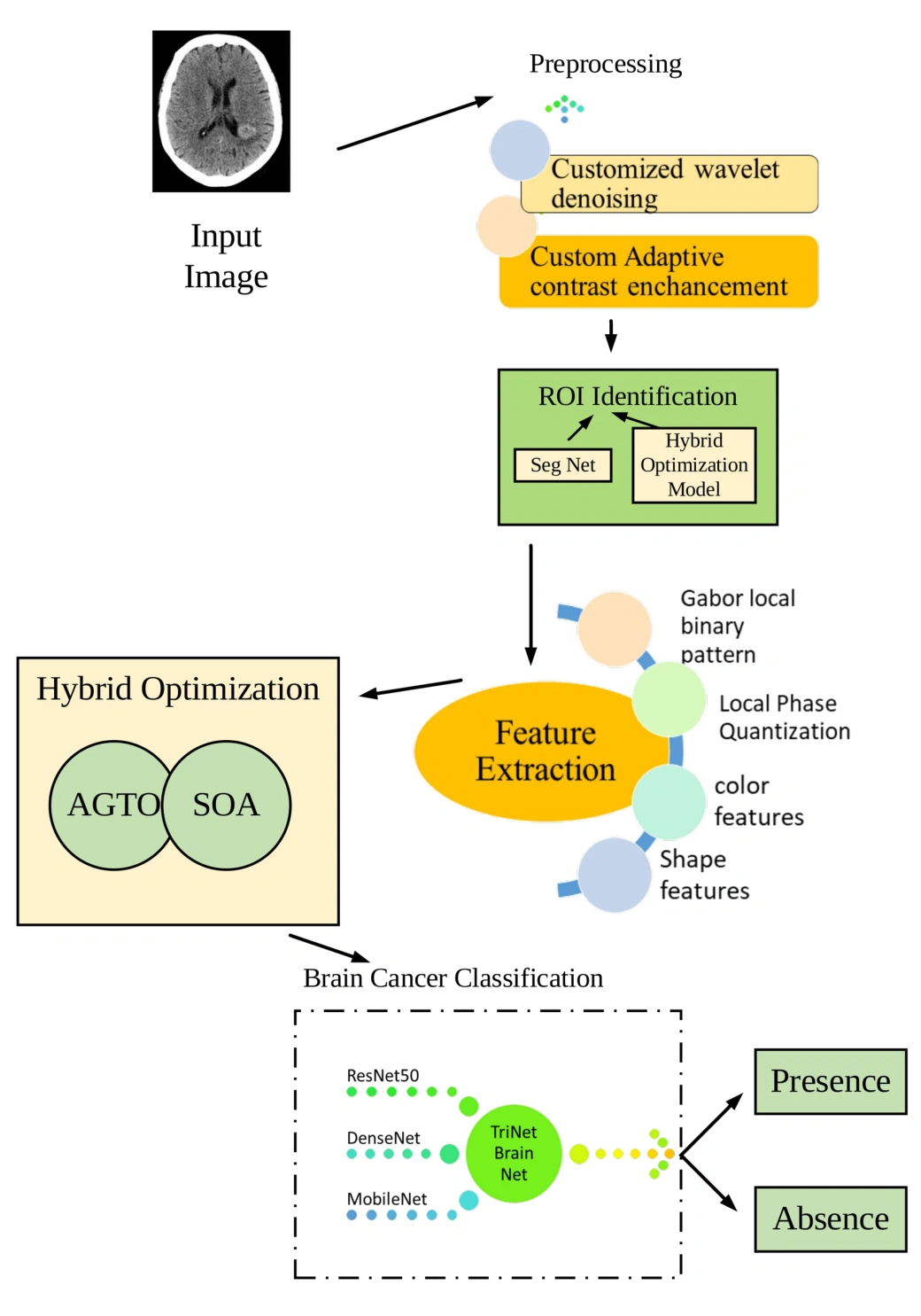
Figure 1: Flow diagram of the proposed model
The flow diagram of the proposed model is shown in Fig.1.
(a) Preprocessing applies customized wavelet denoising and adaptive contrast enhancement to the collected MRI images.
(b) Segmentation identifies regions of interest using optimized SegNet. A hybrid of Artificial Gorilla Troops Optimization and Seagull Optimization tunes the model’s hyperparameters.
(c) Feature extraction derives texture descriptors using Gabor Local Binary Patterns and Local Phase Quantization, colour descriptors using histograms, and shape descriptors using sphericity, elongation, convexity and fractal dimension.
(d) Feature selection uses the hybrid optimisation model to identify relevant descriptors from the extracted feature set.
(e) Classification combines ResNet50, DenseNet and MobileNet in the proposed TriNetX Brain Net weighted voting ensemble.
Preprocessing
Preprocessing applies customized wavelet denoising and adaptive contrast enhancement to prepare the collected MRI images for subsequent segmentation and classification.
Customized Wavelet denoising
The proposed customized wavelet denoising stage reduces noise in the MRI images before contrast enhancement and feature analysis.
Custom Adaptive contrast enhancement for image contrast enhancement
Custom Adaptive Contrast Enhancement using the Contrast Limited Adaptive Histogram Equalization method is a technique designed to enhance image contrast while preventing over-amplification of noise. This process can be explained through a general formula:
 (1)
In this formula:
 represents the adjusted pixel value at coordinates
 in the image after contrast enhancement.
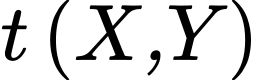 is a transformation function that is applied to each pixel, modifying its intensity.
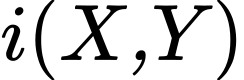 represents the original pixel value at coordinates
 in the image. The key idea here is that the transformation function
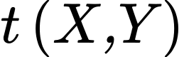 adapts to the local characteristics of the image. It ensures that regions with low contrast are boosted, while regions with high contrast are left relatively unchanged. This adaptability is what sets CLAHE apart. By locally optimizing contrast, it maintains image detail and quality.
This custom adaptive contrast enhancement process, especially when applied to medical images like MRI scans, plays a critical role in improving the clarity and quality of images, making them more suitable for precise brain cancer classification and prediction.
Segmentation
The segmentation stage uses optimized SegNet to identify regions of interest in the preprocessed images. The proposed hybrid model combines Artificial Gorilla Troops Optimization and Seagull Optimization to tune SegNet’s hyperparameters.
Optimized SegNet
SegNet is composed of an encoder, a corresponding decoder network, and a pixel-wise classification layer. The encoder includes 13 convolutional layers, mirroring the initial layers of the VGG16 network designed for object classification. It utilizes pre-trained weights for classification, omitting fully connected layers to maintain higher-resolution feature maps at the deepest encoder output. This reduces the SegNet encoder’s parameter count from 134 million to 14.7 million. Each encoder layer is matched with a decoder layer, resulting in a total of 13 layers in the decoder network. The final decoder output connects to a multi-class softmax classifier, facilitating pixel-wise class probability determination.
SegNet’s decoder network employs a distinct method, involving upsampling input feature maps using the stored max-pooling indices from corresponding encoder feature maps, creating sparse feature maps. These sparse maps undergo convolution with learnable decoder filters, followed by batch normalization. The initial decoder connected to the first encoder generates a multi-channel feature map, differing from the other decoders, which align with their encoder inputs in size and channels. The high-dimensional feature representation from the final decoder is directed to a trainable soft-max classifier for independent pixel-wise classification. The output yields a K-channel image of class probabilities, where K signifies the number of classes. Segmentation predictions are made based on the highest probability class for each pixel.
In the SegNet architectural design, the decoder network employs a unique methodology. It leverages memorized max-pooling indices from the corresponding encoder feature maps to up-sample input feature maps, yielding sparse feature maps. These are subsequently subjected to convolution with trainable decoder filters, followed by batch normalization. Notably, the initial decoder, positioned closest to the input image, generates a multi-channel feature map, even when the input comprises just 3 RGB channels. This contrasts with the other decoders, which maintain consistent size and channel configurations akin to their encoder inputs. The final decoder yields a high-dimensional feature representation, processed by a trainable soft-max classifier for independent pixel-wise classification. The result is a K-channel image representing class probabilities, where K denotes the number of classes. The ultimate segmentation prediction is based on the class with the highest probability for each pixel.

Figure 2: SegNet decoder
Hybrid Simian Aquilla Optimization Algorithm
Artificial Gorilla Troops Optimization models aspects of group behaviour and the role of a dominant silverback. Candidate solutions change position through mathematical update rules representing exploration and exploitation.
The Seagull Optimization Algorithm represents migration and attack behaviour through mathematical search procedures. Position updates model collision avoidance, movement towards promising solutions and spiral attack patterns.
The proposed hybrid combines the two algorithms’ search procedures to balance exploration and exploitation. The following steps describe population initialisation, opposition-based learning, fitness evaluation and position updates.
Step 1: Initialization of population
To initiate the process, an initial population of  search agents is randomly distributed in the search space, representing candidate solutions. Each search agent, denoted as
 , corresponds to the
 individual, where
 signifies the dimension of the search space. The
 dimension of the seagull is generated as follows:
 (2)
In this context, where j varies from 1 to d, the upper limit ( ) and lower limit (
 ) of the dimension determine the range of variation. To populate the initial search agent, each dimension is filled with values using uniformly distributed random numbers within the [0, 1] range. Following this initialization, the search agent population initiates a cyclic search process
Step 2: Oppositional Solution Generation
Opposition-Based Learning, a potent optimization tool has proven instrumental in accelerating the convergence of heuristic optimization methods. OBL’s efficacy lies in evaluating both the current population and an opposing population within the same generation to identify the superior solution for a given problem. This concept has been seamlessly integrated into a multitude of meta-heuristics significantly enhancing convergence rates. To comprehend OBL, it’s essential to establish the concept of opposite numbers as a fundamental component of this innovative approach.  should be a genuine number. The definition of the opposing number
 is
 (3)
The definition may be extended for a D-Dimensional search space as shown below:
 (4)
The point in D-Dimensional search space is  and
 and

In the context of Oppositional Based Optimization, the principles of Opposition-Based Learning find application not only during initialization but also in every iteration, incorporating the concept of the generation jumping rate, denoted as Jr. This dual-phase utilization of OBL contributes to the efficiency and effectiveness of the optimization process.
Step 3: Fitness Computation
The fitness is calculated as
 (5)
Where E is the error.
Step 4: Exploration
In the exploration phase, based on random value r using three strategies as
Strategy (a) 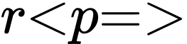 Move towards the other search agent
Strategy (b) 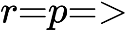 compete with adult search agent
Strategy (c)(i) when 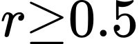 Migrate towards Unknown and (ii) when
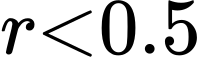 Known position
They are defined as
Strategy (a): Move towards another search agent when 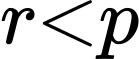
Following Silver back
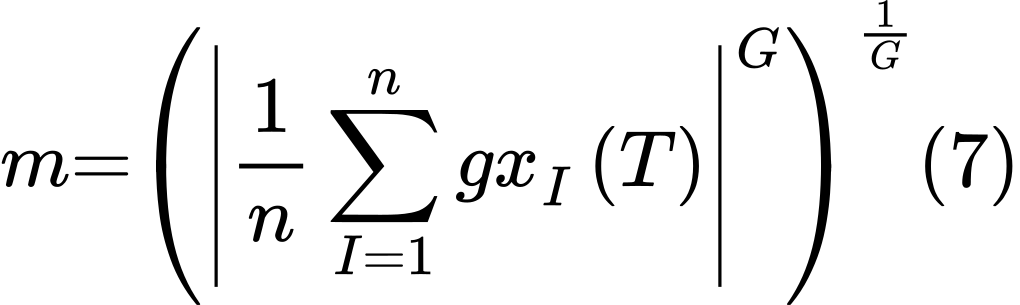
During this stage, two distinct behaviours are observed: following the silverback search agent and competing with adult search agent. In this search agent group, it’s essential to note that these behaviours are separate entities. The parameter C plays a role in determining which strategy male search agent adopt – whether they choose to follow the silverback search agent or engage in competition with other males. Additionally, W, a pre-set parameter, influences this decision-making process. Younger search agents, including males, exhibit a preference for following the silverback search agent as it enhances their performance. Notably, the silverback search agent optimal solution also affects the individual positions of other search agents, influencing their choices and behavior. When C is greater than or equal to W, the policy associated with Eq. (6) is executed.
 (6)
 (8)
where represents the total number of gorillas and  .
Harmonizing Sine and Cosine Functions via Closeness-Based Interaction Fusion Strategy
Recognizing the inherent algorithmic randomness affecting individual search agent positions, a strategy was employed to enhance the algorithm’s exploitation capability. This strategy involved categorizing these positions into “good” and “bad,” subsequently refining individual solutions to boost algorithmic exploitation. The search agent population was segmented based on their proximity to the silverback leader of search agent. The distance between the silverback leader and the search agent with the minimum average closeness was calculated, and this closeness value was then normalized to obtain a parameter termed “Gamma.” A positive Gamma signified a close and stable search agent-silverback relationship, indicating a favourable individual position. Conversely, a negative Gamma implied a more distant and less favourable relationship. The Gamma calculation followed specific procedures to quantify these relationships effectively.
 (9)
 (10)
 (11)
 (12)
In circumstances where a search agent maintains a close relationship with the silverback search agent, considering that even the silverback’s decisions may occasionally err and acknowledging a degree of anthropomorphism, the silverback engages in group communication to align decisions with collective preferences and ensure correctness. This process fuses the optimal individual solution with a randomly generated position, introducing randomness for enhanced exploration while preserving overall population focus. This strategy mitigates blind search and overexploitation. It encourages effective communication between individuals and the silverback, shifting the current solution toward the optimal solution, thus exploring both local and global spaces. A sine-cosine interaction equation with periodic functions supports comprehensive solution exploration. The process is further regulated by a standard normal distribution random number, and the dimension of the problem. When  , priority lies in extensively developing the vicinity to discover superior solutions.
 (13)
 (14)
where  replicates the propensity for group decision-making in gorillas, and its calculation equation is as follows:
 (15)
where, among them, rand is a random number between 0 and 1, mean  refers to the mean vector of all candidate search agent positions, mean
 refers to the mean vector of search agent population positions, and mean
 refers to the mean vector of all search agent positions. Here is the CAN2 calculating equation:
 (16)
In cases of a cold relationship between the silverback and an individual search agent, the silverback aims to dominate, preventing local optima by utilizing sine and cosine functions to relocate to other search agent positions for superior global solutions. This exchange of experience through sine-cosine adjustments is controlled by the parameter CAN3, ensuring efficient behaviour integration.
 (17)
When 
 (18)
 (19)
Strategy (b) Competition with adult female
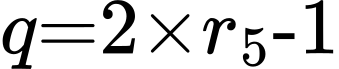
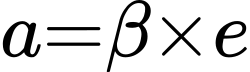
Adolescent search agent prominently engages in fierce and enduring competition for mating opportunities with female search agent. This competition, marked by its intensity and capacity to influence other group members, symbolizes a dynamic exchange of solutions. The competitive interactions reflect the interplay of solutions within the group. Notably, the silverback search agent’s optimal solution shifts towards the positions of other solutions, thus exerting an impact on the current solution, consequently contributing to the pursuit of improved solutions. Eq. (20) effectively models this behaviour in the simulation.
 (20)
 (21)
 (22)
 (23)
where  is a parameter that needs to be set to a certain value before optimization. A random number between 0 and 1 makes up
 .
Avoid collision
In order to prevent collisions with neighbouring seagulls, the algorithm introduces an extra variable, denoted as  , which plays an important role in determining the updated positions of the search agent. This variable helps maintain safe separation and spacing between search agent during their migration process.
 (24)
The variable  signifies a fresh location that ensures no conflicts with other search agent.
 denotes the current position of the search agent, while
 denotes the ongoing iteration. The parameter embodies the behavior of search agent as they navigate within the designated search space, helping them find suitable, non-overlapping positions.
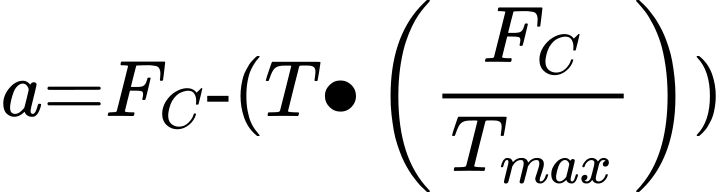 (25)
The parameter  sets the upper limit for the number of iterations.
 modulates the frequency of variable , diminishing linearly from 2 to 0, which regulates search agent behaviour throughout the optimization process.
C(i) Migrate towards unknown position
The specific expression is as follows: After moving to the best place and avoiding overlap with another search agent:
 (26)
The direction of the best location, denoted as 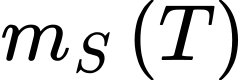 , guides search agent during their movement. The behaviour of
 is intentionally randomized to strike a balance between exploration and exploitation in the optimization process. The calculation of
 is carried out according to a specific algorithm or formula, ensuring adaptive and effective decision-making by the search agent.
C(ii) Migrate towards known places
When a search agent successfully relocates to a collision-free position, it adjusts its trajectory to move closer to the best-positioned search agent to reach its new destination. The formula used to determine the distance between the search agent and the top-performing search agent is expressed as follows:
 (27)
Step 5: Exploitation
Search agent exhibit dynamic control over their attack angle and speed during migration, employing wing adjustments and weight management to sustain their altitude. Their movement resembles a spiral pattern in the air. Their motion behaviour is characterized in the  planes, shaping their trajectory during prey pursuit.
 (28)
 (29)
 (30)
 (31)
The formula determining the search agent attack position is derived from several parameters. It incorporates the radius  of each helix, a random angle value
 within the range [0, 2π], as well as the constants
 affecting the helix shape. Furthermore, the base of the natural logarithm
 is part of the formula, resulting in the precise positioning of search agent during their attack behaviour.
 (32)
 (33)
The search agent attack position during their pursuit of prey is denoted as  . As the iteration count and parameter settings adapt over time, the culmination of their attack behavior leads to the discovery of the global optimal solution. This marks the successful conclusion of the optimization process.
Step 6: Return 

Step 7: Terminate
Feature Extraction
Feature extraction derives texture descriptors using Gabor Local Binary Patterns and Local Phase Quantization, colour descriptors using histograms, and shape descriptors including sphericity, elongation, convexity and fractal dimension.
Gabor Local Binary Pattern
The Gabor Local Binary Pattern is a robust and effective texture feature extraction method commonly used in image analysis and computer vision. GLBP combines the strengths of the Gabor filter, a spatial frequency analysis tool, with the Local Binary Pattern, a texture descriptor. This integration empowers GLBP to encompass texture and spatial data effectively, rendering it well-suited for various tasks like texture classification, face recognition, and object detection.
The GLBP operation can be defined through the following steps and equations:
Gabor Filter Response
In this initial stage, the image is convolved with Gabor filters to extract texture information. The Gabor filter at a specific scale  and orientation is defined as
 (34)
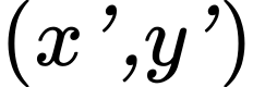 represents the coordinates after rotation;
 is the aspect ratio; σ is the standard deviation;
 is the spatial frequency;
 is the phase offset.
Local Binary Pattern
The Gabor filter responses are employed to apply Local Binary Pattern, encoding connections between the central pixel and its neighbours. It derives a binary pattern by evaluating the intensity relationships between the center pixel and its surrounding pixels, effectively capturing local texture characteristics in the image data.
GLBP Histogram
Finally, a histogram is constructed from the LBP values obtained from the Gabor filter responses. This histogram captures the distribution of texture patterns in the image, effectively summarizing the texture information.
GLBP’s ability to capture both texture and spatial details makes it a valuable tool for a wide range of image analysis tasks, particularly when detailed texture information is crucial for accurate recognition and classification.
Local Phase Quantization
Local Phase Quantization, a texture descriptor in the frequency domain, computes the phase information for pixels within a specified window. LPQ’s notable feature is its blur invariance property, making it valuable for texture classification. To extract features from a Region of Interest (ROI), a short-time Fourier transform (STFT) is applied to the input image  , and a uniform rectangular window
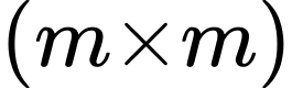 is defined. Within this window, local phase is computed at each pixel location
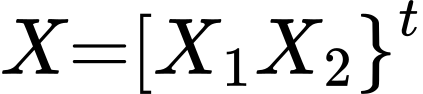 within the neighborhood
 . This 2-D discrete time STFT characterizes the image’s frequency information for further analysis.
 (35)
And  is the 2-D frequency, while
 denotes a window function, which is defined as
 (36)
Phases of four corresponding frequencies are taken into consideration,  , which produce a vector.
 (37)
Using the sign of real and imaginary components, the phase information is further quantized to create an 8-bit binary codeword.
 (38)
And
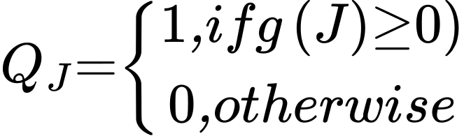 (39)
where  is the quantized version of
 where
 is the component of
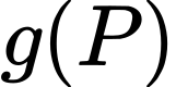 . Q is converted to decimal integers to create the resultant feature vector, which is then shown as a histogram with 256 bins.
Color Features
Color features, specifically color histograms, are vital components in image analysis. They quantitatively represent the distribution of colors in an image, offering insights into its color characteristics. By analysing the frequency of different color values, color histograms provide crucial information for tasks like brain cancer classification, enhancing accuracy and insight.
Color Histogram
The Watershed transform’s outcome is further processed through the calculation of a color histogram in analysis of the brain cancer determining. The input comprises a grayscale image with a single intensity curve, mapping to a 256-level histogram, representing grayscale values ranging from 1 to 255. The exclusion of the zero level signifies the air area. This histogram is presented graphically on a canvas sized at 512 x 400 pixels. This essential step aims to accumulate critical color data from the image, enabling an in-depth description of the image’s color characteristics. It is a valuable asset in subsequent mean value calculations for brain cancer classification.
Shape Features
Shape descriptors represent different geometric properties of the segmented regions. Sphericity measures roundness, elongation describes stretching, convexity compares an object with its convex hull, and fractal dimension describes geometric complexity.
Sphericity
Sphericity, a vital parameter in particle characterization and behaviour, measures a particle’s likeness to a sphere. It’s defined as the ratio of an equal-volume sphere’s surface area to the actual surface area of the particle.
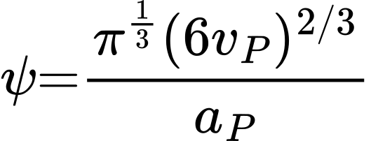 (40)
For irregular particles, sphericity requires an estimate of surface area. The descriptor is used to compare departures from a spherical shape.
Elongation
Elongation is a geometric property that characterizes the degree of stretching or distortion in an object’s shape. It quantifies how much an object deviates from a perfect circle or sphere, often used in image analysis to distinguish between elongated and compact forms, contributing valuable insights across various fields, including materials science and biology.
Convexity
Convexity compares a particle’s area with the area enclosed by its convex hull. The resulting descriptor summarises departures from a convex outline.
Fractal Dimension
Fractal dimension describes how geometric detail changes with the scale of measurement. It provides a way to characterise irregular structures and complex image boundaries.
Brain Tumour Classification with TriNetX Brain Net
The proposed TriNetX Brain Net framework combines ResNet50, DenseNet and MobileNet for brain tumour image classification. Weighted voting combines the component models’ predictions.
ResNet50
Comprising 50 layers organized into five blocks, ResNet-50 employs a series of residual blocks. These innovative blocks enable the retention of valuable information from preceding layers, facilitating improved learning and the acquisition of more meaningful representations from the input data.
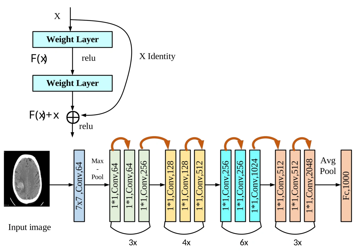
Figure 3: ResNet50 Architecture
ResNet incorporates key components in its architecture.
Convolutional Layer
It commences with convolutional layers, initiating the process of image analysis through convolution operations. Following this, a max-pooling layer is employed to diminish the dimensions of the output originating from the convolutional layer. The streamlined output then progresses through a sequence of residual blocks, allowing for the preservation of crucial information and promoting the learning of intricate representations within the network. This layered approach forms the foundation of ResNet’s remarkable performance in various tasks, including image analysis and recognition.
Residual Block
In ResNet’s structure, the fundamental building block is the residual block, which consists of two convolutional layers, followed by batch normalization and Rectified Linear Unit activation functions. Notably, the output from the second convolutional layer is combined with the input to the block, ensuring the integration of new and existing information. A subsequent ReLU activation further refines the output. This final output is seamlessly transmitted to the following block in the network, enhancing information preservation and fortifying the network’s ability to grasp complex data representations.
Fully connected Layer
The ResNet architecture concludes with a fully connected layer, which plays a role in transforming the final output from the last residual block into discrete output classes. The number of neurons in this layer aligns precisely with the total count of output classes, facilitating the network’s capability to deliver categorical predictions grounded in the acquired features.
Skip connections, recognized as identity connections, play a role in ResNet-50’s architecture. They enable the retention of valuable information from prior layers, enhancing the network’s capability to acquire more meaningful representations from input data. This mechanism is executed by summing the output of an earlier layer with that of a subsequent layer.
DenseNet
In a typical Convolutional Neural Network, the forward pass entails a systematic flow of data from the initial input image towards the ultimate predicted label. This process is characterized by a sequence of convolutional layers, each building upon the feature maps generated by the previous layer. The very first layer is responsible for receiving and processing the input image. Subsequent layers, however, operate in a different manner. They accept the output from the preceding convolutional layer, performing convolutions to produce distinctive output feature maps. Within a CNN consisting of L layers, a total of L direct connections is present, with each layer maintaining a direct link to its immediate successor. This connectivity pattern ensures a seamless propagation of information, allowing the network to progressively uncover and refine intricate hierarchical features, thereby enhancing its capability in tasks like image analysis and classification. The innate design of these direct connections forms the backbone of the network’s effectiveness.
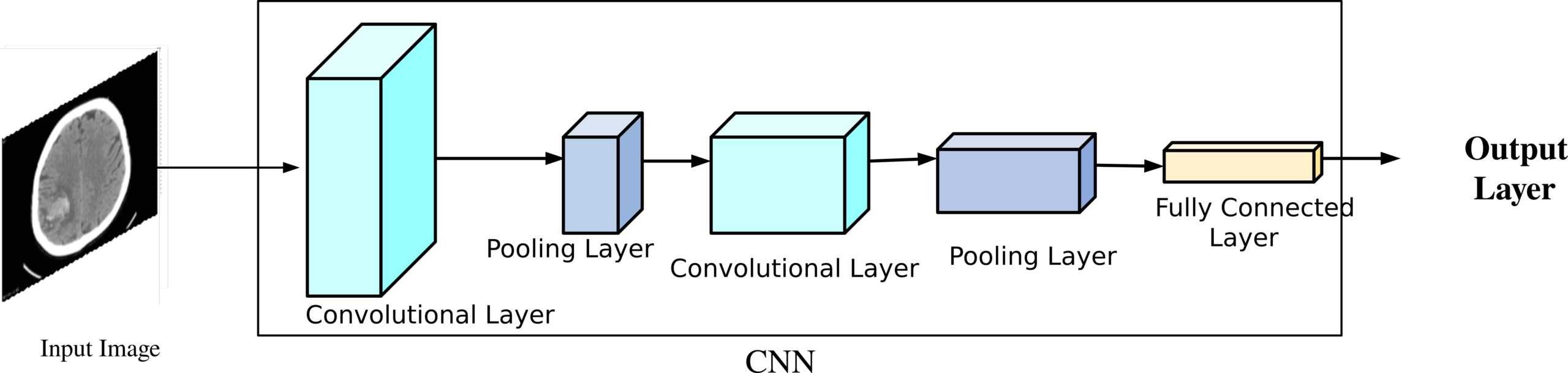
Figure 4: DenseNet Architecture
In the architecture of DenseNet, the essence lies in connecting each layer with every other layer, which gives rise to its name, Densely Connected Convolutional Network. For a network comprising  layers, there are a total of
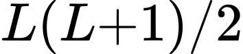 direct connections. In this design, each layer takes not only its own feature maps but also the feature maps from all preceding layers as inputs. Furthermore, its own feature maps are shared with all subsequent layers. This concept, seemingly straightforward, is profoundly powerful. Within DenseNets, a layer’s input is formed by concatenating the feature maps from prior layers, culminating in an interconnected structure that greatly enhances the network’s capacity to learn and extract intricate representations in tasks like image analysis and classification.
MobileNet
MobileNet, initially introduced for mobile and embedded vision applications, forms the basis for efficient and lightweight deep convolutional neural networks. These networks excel in both compact size and rapid performance compared to their larger counterparts. MobileNet relies on depthwise separable convolutions, wherein each input undergoes initial filtering before being combined into a set of output features through 1×1 convolutions.
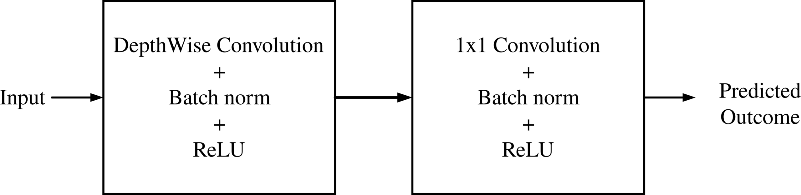
Figure 5: MobileNet Architecture
This approach emulates typical convolution layers but achieves significantly faster processing by dividing the process into two distinct layers: one for filtering and one for combining. This not only reduces model size but also lessens computational requirements, making it a valuable choice for brain cancer prediction. Each layer incorporates batch normalization and ReLU nonlinearity, with the final fully connected layer linking to a softmax layer for classification, devoid of nonlinearity. MobileNet is constructed with 28 layers, not accounting for depthwise and pointwise convolutions, making it an ideal candidate for efficient and accurate brain cancer prediction.
The ensemble combines residual connections from ResNet50, feature reuse from DenseNet and the compact depthwise separable convolutions of MobileNet. These complementary architectures provide the predictions used in the weighted voting stage.
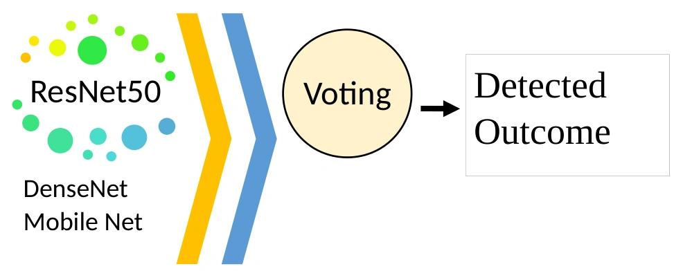
Figure 6: Architecture of TriNetX Brain Net
Weighted voting combines class probabilities from the individually trained ResNet50, DenseNet and MobileNet models. The described approach assigns weights according to validation performance. For each test sample, the weighted probabilities are combined, and the class with the highest resulting probability becomes the final prediction. Standard classification metrics are then used to evaluate the ensemble.
Results and Discussion
Experimental Setup
The manuscript describes implementation in MATLAB and evaluation using accuracy, sensitivity, specificity, precision, true positive rate, false positive rate, true negative rate, F1-score and recall. Comparisons are made with existing models. The dataset is the Brain Tumor MRI Dataset available at https://www.kaggle.com/datasets/masoudnickparvar/brain-tumor-mri-dataset .
Table 2 reports the proposed TriNetX Brain Net model alongside XceptionNet, MobileNet, DenseNet, ResNet and AlexNet. The reported values for the proposed model are sensitivity 0.961, specificity 1, accuracy 0.99, precision 0.98, recall 0.952, F-measure 0.96, negative predictive value 0.96, false positive rate 0.04, false negative rate 0.08 and Matthews correlation coefficient 0.97. The table presents the corresponding values for each comparison model.
Table 2: evaluation of the suggested model’s performance
Models | Sen | Spec | Acc | Precision | Recall | FMeasure | NPV | FPR | FNR | MCC |
Proposed TriNetX Brain Net | 0.961 | 1 | 0.99 | 0.98 | 0.952 | 0.96 | 1 | 0.04 | 0.08 | 0.97 |
XceptionNet | 0.902 | 0.99 | 0.99 | 0.9 | 0.887 | 0.893 | 0.999 | 0.04 | 0.12 | 0.88 |
Mobile Net | 0.861 | 1.01 | 0.97 | 0.88 | 0.876 | 0.872 | 0.998 | 0.04 | 0.16 | 0.84 |
Dense Net | 0.83 | 0.99 | 0.96 | 0.83 | 0.83 | 0.854 | 0.982 | 0.06 | 0.19 | 0.79 |
ResNet | 0.788 | 0.97 | 0.94 | 0.77 | 0.776 | 0.782 | 0.983 | 0.05 | 0.27 | 0.74 |
Alex Net | 0.738 | 0.97 | 0.91 | 0.73 | 0.714 | 0.733 | 0.975 | 0.09 | 0.32 | 0.69 |

Figure 7: Proposed model performance metrics-Sensitivity, Specificity, Accuracy
Figure 7 compares sensitivity, specificity and accuracy for TriNetX Brain Net and the baseline models.
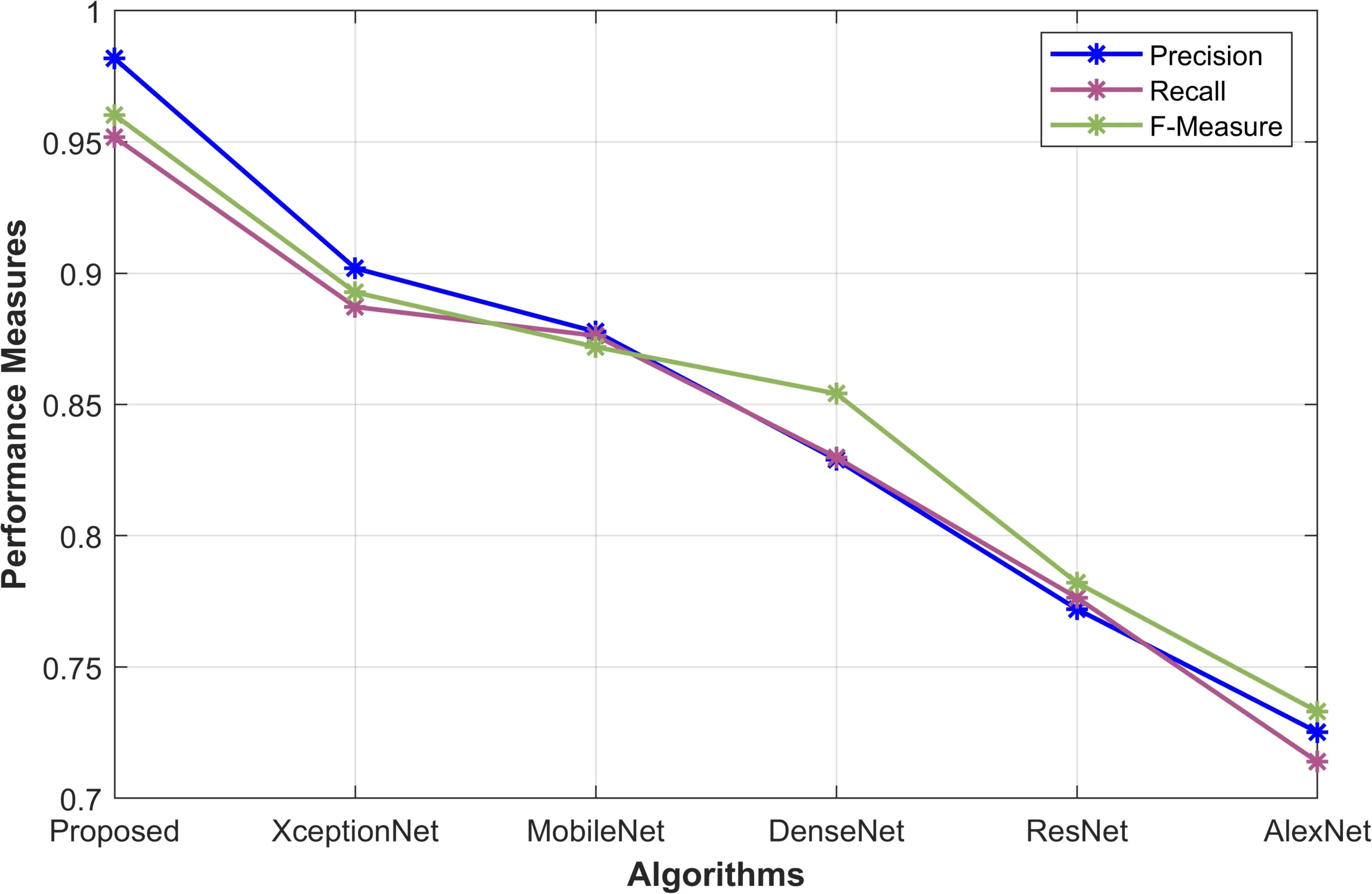
Figure 8: proposed model performance metrics: F-Measure, Precision, and Recall
Figure 8 compares F-measure, precision and recall for the proposed model and the baseline models.
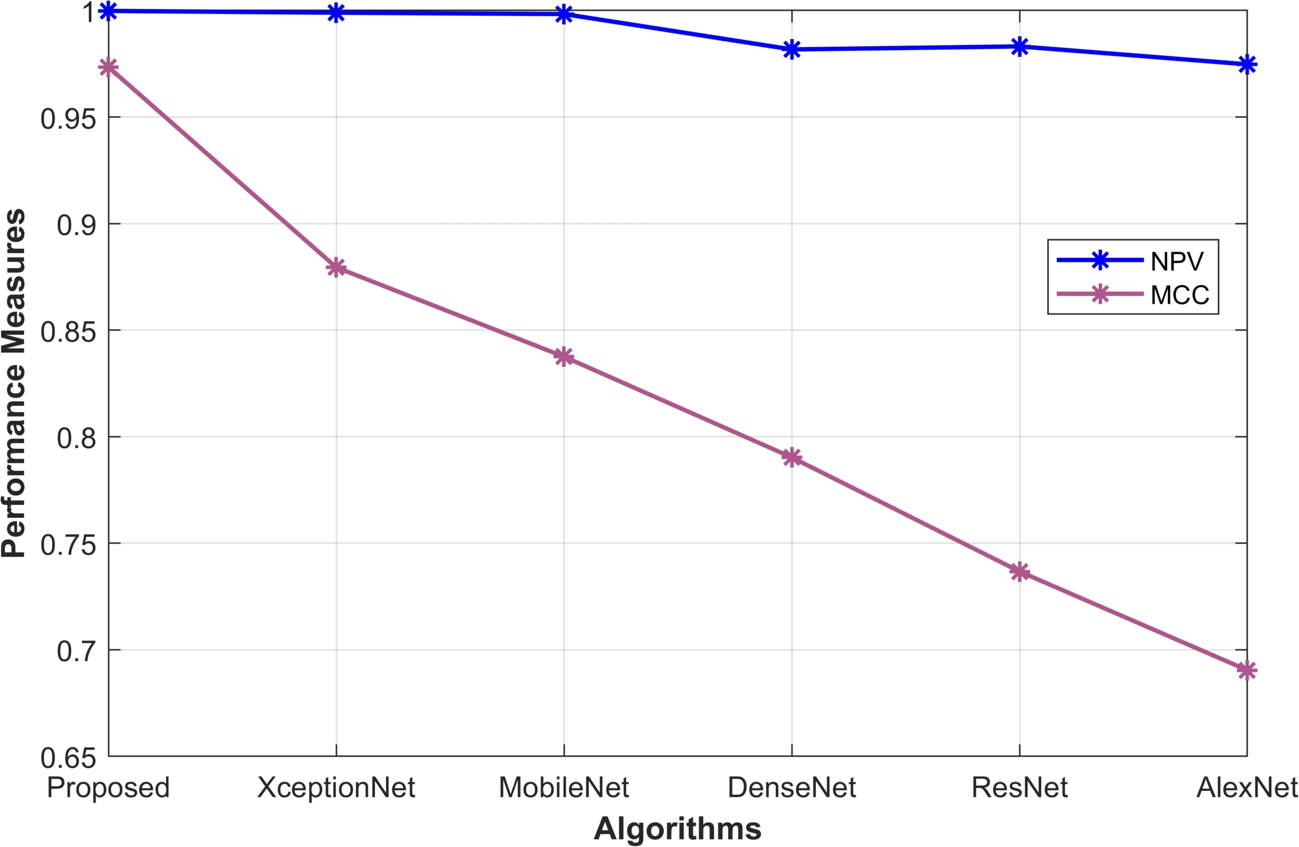
Figure 9: Proposed model performance metrics- NPV, MCC
Figure 9 compares negative predictive value and Matthews correlation coefficient across the evaluated models.
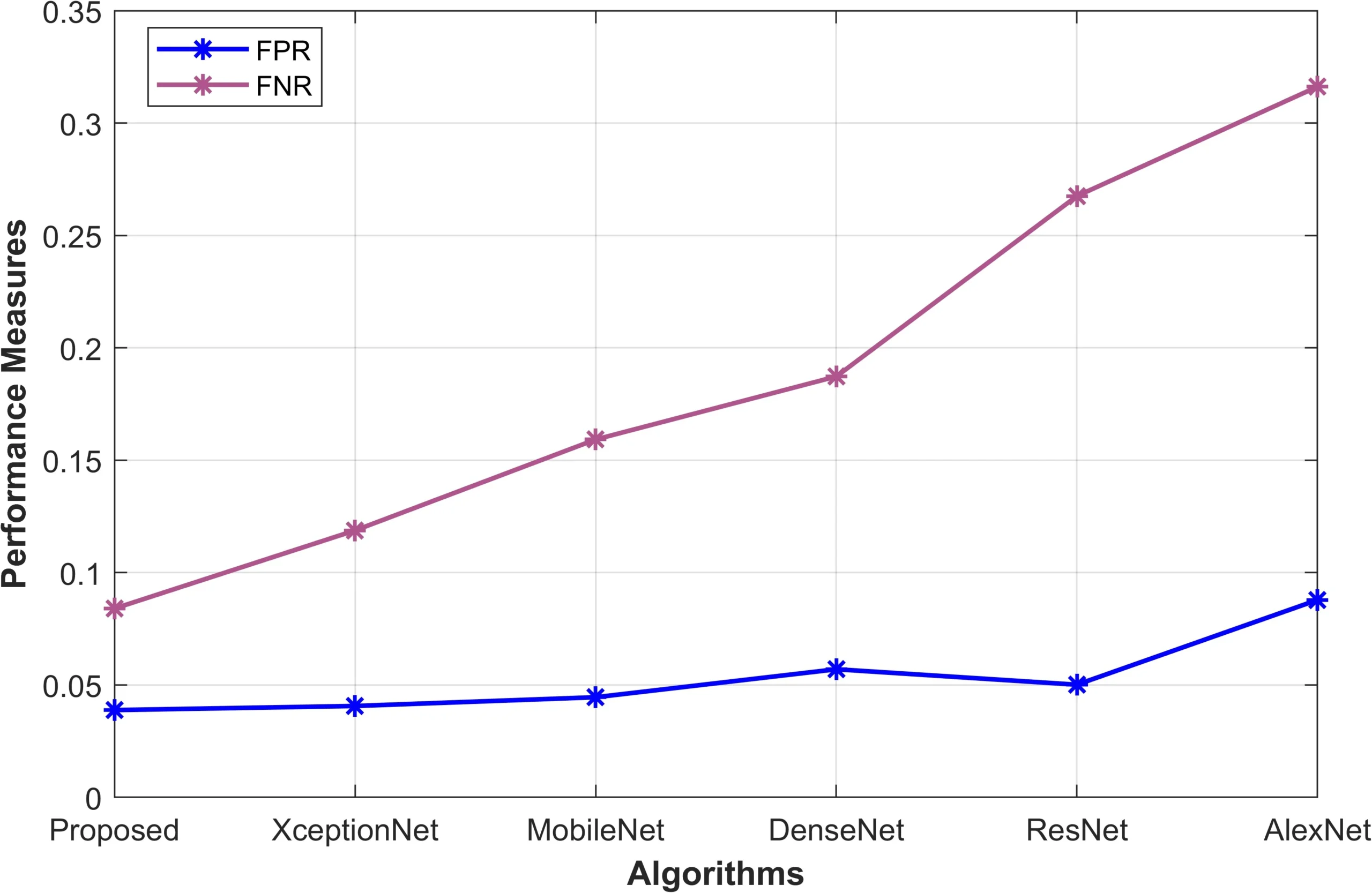
Figure 10: Proposed model performance metrics-FPR, FNR
Figure 10 compares false positive and false negative rates for the proposed model and the baseline models.
|
|
|
|
|
|
|
|
|
|
|
|
|
|
|
Input Image | Pre-processed image | Segmented Image |
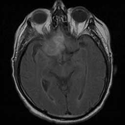

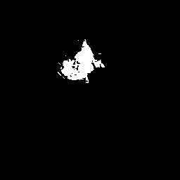


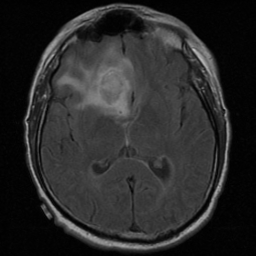


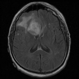


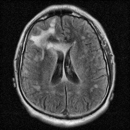
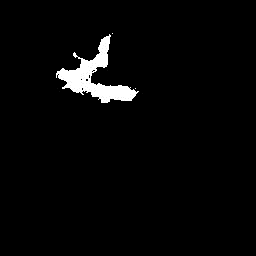
Figure 11: Sample Input images and its pre-processed and its segmented image
Conclusion
The study presents a five-phase framework for brain tumour image classification: preprocessing, segmentation, feature extraction, feature selection and classification. Customized wavelet denoising and adaptive contrast enhancement prepare the MRI data. Optimized SegNet identifies regions of interest, with its hyperparameters tuned by the author-defined Simian Aquilla Optimization Algorithm combining Artificial Gorilla Troops Optimization and Seagull Optimization. Texture, colour and shape descriptors characterise the segmented regions, and the hybrid optimiser selects relevant features. TriNetX Brain Net combines ResNet50, DenseNet and MobileNet to produce the final predictions. The manuscript describes a MATLAB implementation using the cited Kaggle dataset and compares the proposed system with existing models through classification metrics and illustrated examples. These reported experiments describe the computational framework’s performance on the study data.
References
Amin, J., Sharif, M., Yasmin, M. and Fernandes, S.L., 2020. A distinctive approach in brain tumor detection and classification using MRI. Pattern Recognition Letters, 139, pp.118-127.
Khairandish, M.O., Sharma, M., Jain, V., Chatterjee, J.M. and Jhanjhi, N.Z., 2022. A hybrid CNN-SVM threshold segmentation approach for tumor detection and classification of MRI brain images. Irbm, 43(4), pp.290-299.
Rajesh, T., Malar, R.S.M. and Geetha, M.R., 2019. Brain tumor detection using optimisation classification based on rough set theory. Cluster computing, 22(Suppl 6), pp.13853-13859.
Saba, T., Mohamed, A.S., El-Affendi, M., Amin, J. and Sharif, M., 2020. Brain tumor detection using fusion of hand crafted and deep learning features. Cognitive Systems Research, 59, pp.221-230.
Amin, J., Sharif, M., Raza, M., Saba, T., Sial, R. and Shad, S.A., 2020. Brain tumor detection: a long short-term memory (LSTM)-based learning model. Neural Computing and Applications, 32, pp.15965-15973.
Özyurt, F., Sert, E., Avci, E. and Dogantekin, E., 2019. Brain tumor detection based on Convolutional Neural Network with neutrosophic expert maximum fuzzy sure entropy. Measurement, 147, p.106830.
Mohsen, H., El-Dahshan, E.S.A., El-Horbaty, E.S.M. and Salem, A.B.M., 2018. Classification using deep learning neural networks for brain tumors. Future Computing and Informatics Journal, 3(1), pp.68-71.
Nabizadeh, N. and Kubat, M., 2015. Brain tumors detection and segmentation in MR images: Gabor wavelet vs. statistical features. Computers & Electrical Engineering, 45, pp.286-301.
Abiwinanda, N., Hanif, M., Hesaputra, S.T., Handayani, A. and Mengko, T.R., 2019. Brain tumor classification using convolutional neural network. In World Congress on Medical Physics and Biomedical Engineering 2018: June 3-8, 2018, Prague, Czech Republic (Vol. 1) (pp. 183-189). Springer Singapore.
Raja, P.S., 2020. Brain tumor classification using a hybrid deep autoencoder with Bayesian fuzzy clustering-based segmentation approach. Biocybernetics and Biomedical Engineering, 40(1), pp.440-453.
Bargaje, A., Kulkarni, A. and Lagad, S., 2017. Brain tumor detection and classification using adaptive boosting. International Research Journal of Engineering and Technology (IRJET), 4(7), pp.1961-1965.
Irmak, E., 2021. Multi-classification of brain tumor MRI images using deep convolutional neural network with fully optimized framework. Iranian Journal of Science and Technology, Transactions of Electrical Engineering, 45(3), pp.1015-1036.
Rehman, A., Naz, S., Razzak, M.I., Akram, F. and Imran, M., 2020. A deep learning-based framework for automatic brain tumors classification using transfer learning. Circuits, Systems, and Signal Processing, 39, pp.757-775.
Amin, J., Sharif, M., Gul, N., Yasmin, M. and Shad, S.A., 2020. Brain tumor classification based on DWT fusion of MRI sequences using convolutional neural network. Pattern Recognition Letters, 129, pp.115-122.
Sultan, H.H., Salem, N.M. and Al-Atabany, W., 2019. Multi-classification of brain tumor images using deep neural network. IEEE access, 7, pp.69215-69225.
Varuna Shree, N. and Kumar, T.N.R., 2018. Identification and classification of brain tumor MRI images with feature extraction using DWT and probabilistic neural network. Brain informatics, 5(1), pp.23-30.
Kaplan, K., Kaya, Y., Kuncan, M. and Ertunç, H.M., 2020. Brain tumor classification using modified local binary patterns (LBP) feature extraction methods. Medical hypotheses, 139, p.109696.
Khan, M.A., Ashraf, I., Alhaisoni, M., Damaševičius, R., Scherer, R., Rehman, A. and Bukhari, S.A.C., 2020. Multimodal brain tumor classification using deep learning and robust feature selection: A machine learning application for radiologists. Diagnostics, 10(8), p.565.
Deepak, S. and Ameer, P.M., 2019. Brain tumor classification using deep CNN features via transfer learning. Computers in biology and medicine, 111, p.103345.
Ismael, S.A.A., Mohammed, A. and Hefny, H., 2020. An enhanced deep learning approach for brain cancer MRI images classification using residual networks. Artificial intelligence in medicine, 102, p.101779.
Sajjad, M., Khan, S., Muhammad, K., Wu, W., Ullah, A. and Baik, S.W., 2019. Multi-grade brain tumor classification using deep CNN with extensive data augmentation. Journal of computational science, 30, pp.174-182.
Raza, A., Ayub, H., Khan, J.A., Ahmad, I., S. Salama, A., Daradkeh, Y.I., Javeed, D., Ur Rehman, A. and Hamam, H., 2022. A hybrid deep learning-based approach for brain tumor classification. Electronics, 11(7), p.1146.
Kang, J., Ullah, Z. and Gwak, J., 2021. Mri-based brain tumor classification using ensemble of deep features and machine learning classifiers. Sensors, 21(6), p.2222.
Ghassemi, N., Shoeibi, A. and Rouhani, M., 2020. Deep neural network with generative adversarial networks pre-training for brain tumor classification based on MR images. Biomedical Signal Processing and Control, 57, p.101678.
Özyurt, F., Sert, E. and Avcı, D., 2020. An expert system for brain tumor detection: Fuzzy C-means with super resolution and convolutional neural network with extreme learning machine. Medical hypotheses, 134, p.109433.
National Cancer Institute. (n.d.). Adult Central Nervous System Tumors Treatment (PDQ®). https://www.cancer.gov/types/brain/patient/adult-brain-treatment-pdq
Cite This Work
To export a reference to this article please select a referencing stye below:

Academic Master Education Team is a group of academic editors and subject specialists responsible for producing structured, research-backed essays across multiple disciplines. Each article is developed following Academic Master’s Editorial Policy and supported by credible academic references. The team ensures clarity, citation accuracy, and adherence to ethical academic writing standards
Content reviewed under Academic Master Editorial Policy.