
Abstract
This study presents a deep learning framework for assessing physical rehabilitation exercises using the KIMORE dataset. Preprocessing prepares skeleton joint-position data, while Generative Adversarial Networks augment the training material. Contrast Limited Adaptive Histogram Equalization enhances the resulting images. Joint-level, limb-level, temporal and statistical descriptors provide features for movement assessment. The proposed Coati Predator Optimization Algorithm combines Coati Optimization and Marine Predators Optimization to select relevant features and support hyperparameter tuning. The learning framework combines a Multilayer Perceptron, an attention-based Convolutional Neural Network and a Recurrent Neural Network, with transfer learning. Grad-CAM visualisations provide graphical explanations of model outputs. The manuscript reports exercise-specific comparisons with baseline models to examine the framework’s classification performance.
Keywords: Generative Adversarial Networks, CLAHE; Coati Optimization Algorithm; Marine Predators Algorithm; Multilayer Perception;Recurrent Neural Network, Transfer Learning, Attention-based Convolutional Neural Network.
Introduction
Physical activity and exercise received renewed attention during the COVID-19 pandemic because of their relationship with physical and mental well-being [1]. Task-specific exercises are used in musculoskeletal assessment and post-stroke rehabilitation [2]. Tailored rehabilitation can support physical activity and daily functioning in older adults [3]. Physical activity is also associated with cardiovascular factors such as weight, blood pressure and insulin sensitivity [4]. Postoperative rehabilitation, including rehabilitation after joint surgery, requires reliable assessment. Computational models may support monitoring, adherence and access to rehabilitation services [5][6].
Ageing, injury and cognitive decline can affect posture and gait. Rehabilitation assessment examines whether movement practice corresponds to an individual’s recovery needs. Walking activities and real-time review may support work on gait and postural stability [7][8]. Pulmonary rehabilitation addresses physical and psychosocial needs in chronic respiratory conditions. Neurological rehabilitation also draws on the nervous system’s capacity to adapt during recovery [9][10].
A progressive rehabilitation intervention addressing several physical-function domains improved outcomes in older patients hospitalised with acute decompensated heart failure compared with standard care [11]. Research has also examined relationships between physical exercise and mental well-being [12]. Ensemble classification and deep learning provide methods for recognising actions from sensor data [13]. Rehab-Net uses a low-complexity convolutional architecture with pooling and a fully connected layer [14]. Graph-structured data introduce additional modelling challenges because their relationships differ from those in regular image grids [15].
The main contributions of this research are as follows:
To preprocess skeleton data using GAN-based augmentation and CLAHE.
To extract joint-level, limb-level, temporal and statistical features from the preprocessed data.
To select relevant features using the proposed Coati Predator Optimization Algorithm, combining Coati Optimization and Marine Predators Optimization.
To develop a three-layer deep learning architecture for movement assessment using an optimized MLP, an attention-based CNN and an RNN, together with transfer learning.
To tune the proposed MLP’s hidden layers using the hybrid Coati Predator Optimization Algorithm.
To include Grad-CAM visualization to show graphical explanations for the model’s conclusions.
The research follows a well-organized format: Section 1 introduces the research, Section 2 explores an overview of literature, Section 3 provides specifics about the suggested methodology, Section 4 presents the findings and engages in discussions, and Section 5 summarizes the overall conclusions and results.
Literature Review
In 2020, Liao et al. [16], introduced a deep learning-based framework for the automated evaluation of physical rehabilitation exercise quality. The framework consisted of metrics that quantified movement performance, scoring functions that converted these metrics into numerical quality scores, and deep neural network models that generated quality assessments for input movements through supervised learning.
In 2022, Kanade et al. [17] proposed a recent deep learning advancements to tackle the challenge of assessing movement quality. It introduced an innovative transformer-based architecture for Movement Quality Assessment (MQA) and incorporated the attention mechanism into the proposed feature design. This approach aimed to enhance the accuracy and effectiveness of movement quality scoring.
In 2018, Capecci et al. [18] introduced a Hidden Semi-Markov Model (HSMM) based approach that was employed for the evaluation and monitoring of body motion in a rehabilitation training program. This approach integrated various facets of rule-based and template-based methods, offering a comprehensive and effective means of assessing and tracking body movements during the program.
In 2020, Caru et al. [19] concluded by examining the impact of a rehabilitation program on both physiological and psychological parameters, with a specific focus on comparing depression scores among different scales. Cardiovascular diseases remained a leading global cause of mortality. The utilization of exercise-based rehabilitation in cardiac patients continued to gain prominence as an effective approach.
In 2018, Mandolesi et al. [20] proposed the biological and psychological benefits of physical exercise (PE), elucidating outcomes from studies in animals and humans that explored brain plasticity and epigenetic mechanisms. The goal was to elucidate strategies for optimizing PE’s positive impact while mitigating potential adverse effects, such as exercise addiction.
In 2022, Rahman et al. [21] introduced an automated method for identifying various therapy exercises executed by stroke patients in their rehabilitation routines. Detecting these exercises posed a challenge in human activity recognition. Leveraging the advancements in deep learning, the research presented a DL model, named the 3-Layer CNN-LSTM model, which integrated convolutional neural networks and long short-term memory to enhance accuracy and efficacy.
In 2020, Schez-Sobrino et al.[22] introduced a computer vision-based system designed for home-based use, enabling automated assessment of exercise performance with data transmission to healthcare facilities. Gamification strategies engaged patients during rehabilitation exercises. Additionally, a distributed gamified system was proposed, which automatically evaluated exercise performance by analyzing and comparing motion curves using the Dynamic Time Warping (DTW) algorithm.
In 2019, Iwao et al. [23] investigated the efficacy of a comprehensive, long-term care prevention program for enhancing the well-being of older adults living in the community. This program integrated physical exercise, oral health guidance, and nutritional counseling to promote the health and quality of life of this population.
In 2021, Whyte et al. [24] summarized the recommendations proposed by a working group, with the objective of improving the reporting of rehabilitation treatments. These suggestions were intended to be integrated with the efforts of multiple working groups, employing a consensus-based process, to develop comprehensive reporting guidelines for randomized controlled trials in the realm of physical medicine and rehabilitation.
In 2018, Van der windt et al. [25] provided substantial evidence regarding the impact of physical exercise on Non-alcoholic Fatty Liver Disease (NAFLD) and Non-alcoholic Steatohepatitis (NASH). Multiple clinical trials affirmed that both aerobic and resistance exercises effectively lowered hepatic fat levels. Furthermore, findings from clinical and fundamental research underscored the multifaceted pathways through which exercise influenced fatty liver disease.
Problem Statement
Author | Methodology | Advantage | Disadvantage |
Zhang et al. [4] | Physical Exercise | Physical exercise can lead to Improving creativity, Boosting the mind, Building agility, etc. | Too much exercise can lead to Physical burnout, Hormonal dysfunction, etc. |
Rochester et al. [9] | Pulmonary Rehabilitation (PR) | enhances physical fitness, lessens anxiety or depressive symptoms, and makes it simpler to handle daily tasks, work, and social outings. | It is not suitable for people with unstable cardiac disease, who easily get short of breath |
Panwar et al. [14] | Convolutional Neural Network (CNN) | No need for human supervision, Automatic feature extraction, Highly accurate at image recognition & classification, Weight sharing | They need a lot of labeled data to train efficiently, but getting and annotating that data can be expensive and time-consuming. |
Liao et al. [16] | Deep Learning (DL) | Enables machines to become more advanced. | Requires a very large amount of data to perform better than other techniques |
Capecci et al. [18] | Hidden Semi-Markov Model (HSMM) | They can capture the probabilistic dependencies between the observed features and the underlying states of a system, and allow for efficient inference and learning algorithms. | It cannot be the true model of the underlying situation in most cases |
Rahman et al. [21] | Human Activity Recognition (HAR) and Long Short-Term Memory (LSTM) | HAR can provide real-time insights into what persons are doing (walking, running, driving, etc.). LSTM is much better at handling long-term dependencies | In HAR computational complexity will be more if the number of layers is increased. LSTM is not easy to parallelize during training. |
Schez-Sobrino et al. [22] | Dynamic Time Warping (DTW) | Between reference and test patterns, accurate time alignment is attained. | The best time alignment path must be discovered through a significant computational effort. |
Proposed Methodology
The proposed framework assesses multimodal human movement using the KIMORE dataset. Preprocessing prepares skeleton joint-position images. GAN-based augmentation expands the training material, and CLAHE enhances image contrast. Joint-level, limb-level, temporal and statistical features represent the input. The proposed Coati Predator Optimization Algorithm combines Coati Optimization and Marine Predators Optimization for feature selection and model tuning. The learning framework includes an optimized MLP, an attention-based CNN and an RNN, together with transfer learning. Grad-CAM visualisation supports interpretation of model outputs. Figure 1 summarises the workflow.
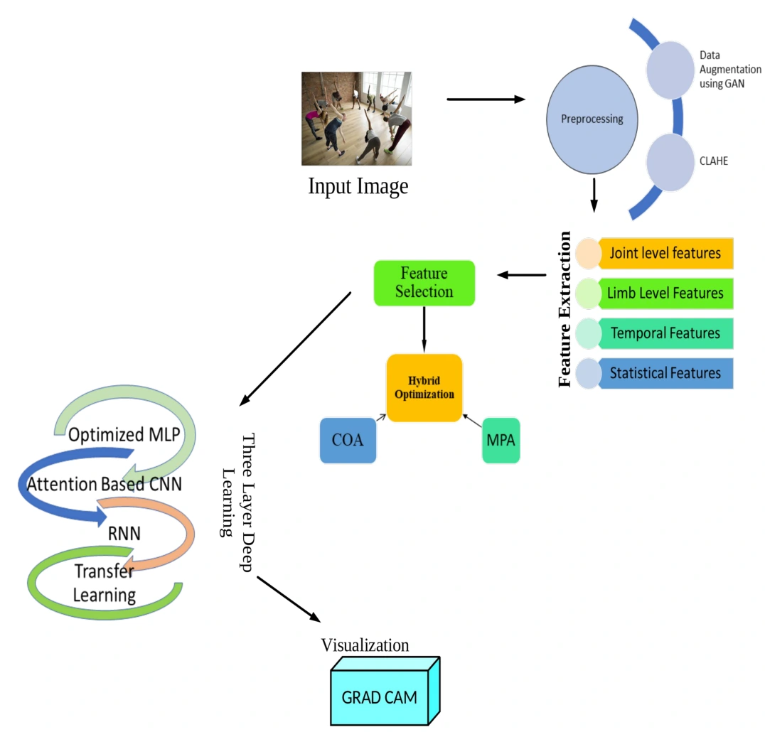
Figure 1: The proposed model’s process diagram
Image Preprocessing
Preprocessing prepares consistent skeleton joint-position images. GAN-based skeleton augmentation expands the training material, and CLAHE enhances image contrast before feature extraction.
Data augmentation
Data augmentation is a method that involves expanding the training dataset artificially by generating altered versions of existing data. This can involve introducing subtle variations to the original dataset or employing deep learning techniques to produce entirely new data points, ultimately enriching the training set for improved model performance.
Skeleton Augmentation using GAN
Only a limited amount of alternative data is generated by conventional augmentation methods. Additionally, Generative Adversarial Networks (GANs) are used for data augmentation in which they produce copies of the original image and which can be used to create a big data set. Without explicated training data, GANs can learn deep representations. GANs are made up of two neural networks, the discriminator and the generator, as depicted in Fig (2) . The Generator (G) will try to generate the replica while learning from the data distributions provided. The Discriminator (D) will determine whether the generated copy of data is real or fake, that is, whether the input data comes from the genuine training dataset or from the generator. When the Discriminator finds the fake data. It will be returned to the generator. The Generator will attempt to provide more realistic data after learning from the loss function. The process will repeat until the Discriminator is unable to tell the difference between actual and fake data.
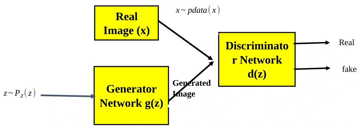
Figure 2: Architecture of GAN
CLAHE
The Contrast Limited Adaptive Histogram Equalization method processes localized image sections, referred to as tiles, rather than the entire image. It alleviates artificial seams between adjacent tiles by employing bilinear interpolation. This technique is particularly effective in enhancing image contrast. For color images, it’s typical to apply this method to the luminance channel in the HSV color space. Remarkably, equalizing only the luminance channel within an HSV image often outperforms equalizing all channels in a standard BGR image.
Feature Extraction
The proposed feature extraction process encompasses various aspects, including Limb and joint level Features, Temporal Features, and Statistical Features. This comprehensive approach involves capturing nuanced information such as mean, range, variance, and standard deviation of both joint and limb angles, facilitating a robust characterization of the data.
Joint Level Features
In image processing, joint-level features pertain to attributes or characteristics extracted from pairs or groups of pixels or image regions, rather than individual pixels. These features capture relationships, patterns, and interactions between different parts of an image. For example, co-occurrence matrices are used to compute texture features by analyzing pixel pairs’ spatial relationships. Joint histograms represent the relationships between color channels in color images. Such joint-level features are crucial for tasks like image segmentation, object recognition, and texture analysis, as they capture higher-level information about image content and structure.
Limb-Level Features
In image processing, limb-level features refer to characteristics extracted from specific regions or structures within an image, such as individual limbs or body parts in a human or animal subject. These features are used for tasks like object recognition and pose estimation, focusing on fine-grained details within the image.
Temporal Features
Temporal features in deep learning refer to patterns or information that evolve over time. They are crucial for tasks like video analysis, speech recognition, and time-series forecasting. Models like recurrent neural networks and transformers capture these temporal dependencies, enabling better understanding and prediction of sequential data.
Statistical Features
Mean and variance
To determine the pixel sum, divide the values by the total pixel count. Each pixel in a computer-stored image carries information about its brightness or color. The mean value represents how each pixel contributes to the overall intensity of the image, while variance is typically used to determine how each pixel differs from the center pixel or nearby pixels and is used to categorize the image into distinct regions.
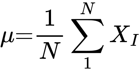 (1)
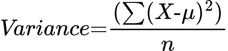 (2)
Where the number of terms in distribution is represented as n ;  is the mean.
Range
The range of your data in statistics is the range from the distribution’s lowest value to its highest value. It serves as a typical indicator of unpredictability. measurements of variability provide descriptive statistics for your data set’s summary, together with measurements of central tendency.
 (3)
R refers the range ;
Standard Deviation of Joint angles
The Standard Deviation of joint angles in image processing is a statistical measure that quantifies the variability or dispersion of joint angles within a set of data points, often used in tasks like pose estimation. The formula for calculating the standard deviation 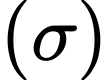 of a set of joint and limb angles (
 is as follows:
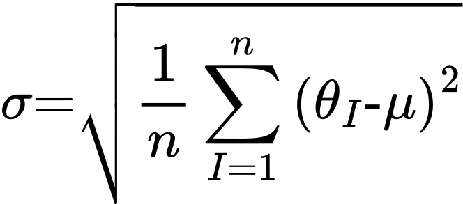 (4)
Where:
 is the number of joint and limb angle measurements.
 represents individual joint and limb angle values.
 is the mean (average) of the joint and limb angle values.
This formula calculates the spread or deviation of joint and limb angles from their mean, providing insight into the overall variability of the pose.
Feature Selection via Coati Predator Optimization Algorithm
The proposed Coati Predator Optimization Algorithm (CPOA) selects features by combining the Coati Optimization Algorithm (COA) and Marine Predators Algorithm (MPA).
COA models the behaviour of coatis, members of the Procyonidae family. Its search procedures draw on cooperative hunting and responses to predators. The algorithm represents these behaviours as position updates within a search space.
MPA, a novel algorithm, emulates the hunting behaviors of marine predators during prey pursuit. It encapsulates the foraging strategies of these predators, relying on two distinct random walk patterns: the Lévy flight and Brownian motion. These strategies enable MPA to explore search spaces and navigate through optimization problems, drawing inspiration from the efficient hunting tactics observed in marine predators.
The hybrid design combines complementary search procedures to balance exploration and exploitation and reduce the likelihood of remaining in local optima.
Step 1 Initialization Method
The COA method, a population-based metaheuristic, utilizes search agents as essential algorithm components. These agents’ positions in the search space encode potential solutions based on decision variable values. To initiate COA, search agents’ positions in the search space are randomly initialized, as described by Eq (5). This initialization process sets the stage for the algorithm to embark on its optimization journey, utilizing the unique attributes of the search agent to explore and improve candidate solutions efficiently.
 (5)
Within the COA algorithm,  denotes the Ith search agent’s location in the search space, with
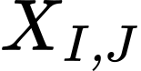 indicating the value of the
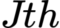 decision variable.
 represents the search agent population size, “m” is the count of decision variables, and
 stands for a randomly generated real number within the [0, 1] range. Furthermore,
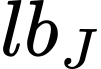 and
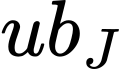 ” symbolize the lower and upper bounds for the
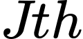 decision variable, respectively.
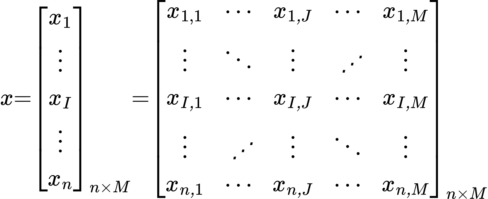 (6)
In COA, the population of search agent is mathematically depicted by the population matrix  .
Step 2 Fitness Computation
The fitness is calculated as follows
 (7)
Where A is the accuracy. Utilizing fitness calculations, solutions are categorized as Elite and Prey. Hence, the most optimal solutions are embodied by the most adept search agent, contributing to the creation of the Elite matrix, as outlined below.
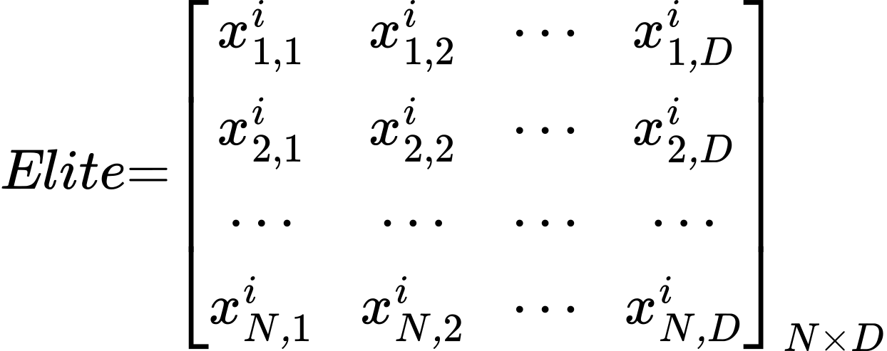 (8)
Here,  denotes the vector of the most adept search agent, which is iteratively multiplied
 times to construct the Elite matrix. Here,
 represents the number of searching agents, and
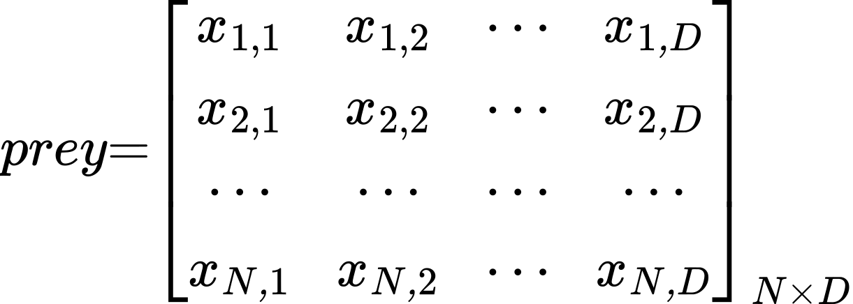
 signifies the dimensionality of the problem. The Elite matrix arrays serve to locate prey based on their positions. It is essential to note that both search agent and prey are considered searching agents within this context. Additionally, a novel matrix, referred to as “Prey,” is established with dimensions mirroring those of the Elite matrix. This Prey matrix plays a role in the overall algorithm.
 (9)
Step 3 Solution Updating
(a) 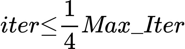
Phase 1 of the COA algorithm, known as the exploration phase, emulates search agent’ hunting when attacking prey strategy. In this phase, a subset of search agent climbs trees to frighten the prey, while others wait beneath for the prey to descend. Once the prey reaches the ground, search agent jointly pursue and capture it. This dynamic strategy results in search agent moving Demonstrating COA’s capacity for global exploration by relocating within the search space. The best population member’s position is equated with the prey’s location, with half of the search agent ascending trees and the other half remaining on the ground. Mathematically, the positions of climbing search agent are calculated using Eq. (10), effectively replicating this hunting pattern.
 (10)
Once the prey descends to the ground, it undergoes a random relocation within the search space, exemplifying dynamic adaptability. Search agent on the ground subsequently adjust their positions in response to this new prey location, a process mathematically represented by Eq. (11) and (12). This adaptation reflects the search agents hunting dynamics in the COA algorithm.
 (11)
 (12)

In the update procedure for each search agent, the assessment checks if the newly computed position improves the objective function’s value. If it does, the search agent adopts the new position; otherwise, it retains its prior position. This update condition applies to search agent indexed from 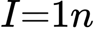 and is expressed in Eq.(13).
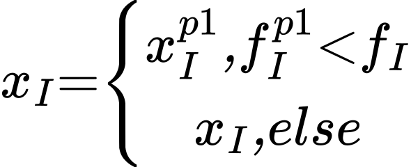 (13)
In the equation, 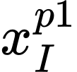 represents the newly calculated position for the
 search agent, with
 denoting its
 dimension.
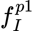 corresponds to the search agent objective function value. The decision to accept this new position depends on a random real number
 in the [0, 1] interval, with comparison to the prey’s position
 represented as the best member’s location.
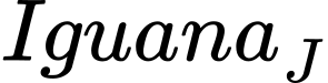 signifies the jth dimension of the prey’s position, and I is a randomly chosen integer from {1, 2}. The ground-based prey position
 and its objective function value
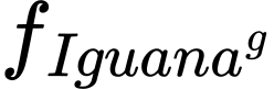 are also factors considered, with
 representing the floor function.
(b) 
In scenarios with a high-velocity ratio  the predator outpaces its prey. This phase emerges during the exploration phase iterations and is characterized by a specific mathematical model.
 (14)
 (15)
In this algorithm, R is a vector with random values between 0 and 1, and  denotes element-wise multiplication.
 is set to 0.5, and , while ‘N’ determines population size.
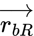 is a vector derived from gradient motion, while
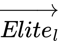 is a matrix storing the fittest solution, serving as a top search agent. Prey motion is governed by the product of
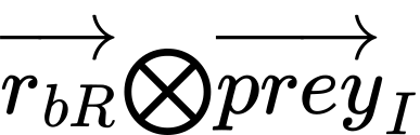 , where
 remains a constant set to 0.5.
 represents a vector of uniformly distributed random numbers ranging from 0 to 1. In this context, 𝐼𝑡𝑒𝑟 signifies the current iteration, while 𝑀𝑎𝑥_𝐼𝑡𝑒𝑟 denotes the maximum iteration limit.
( c) 
During the exploitation phase, the search agent exhibits heightened speed compared to the prey. It strategically employs a Lévy flight maneuver to seize the prey, marking an exploitative strategy. This phase unfolds within the final third of the total iterations, with its dynamics mathematically represented for precise modeling.
 (16)
 (17)
The search agents’ motion, following the Lévy strategy, can be expressed as the product of 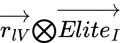 . To enhance the prey position update, the search agent motion is further characterized by adding a step size to the Elite position, contributing to the refinement of the overall search agent strategy.
(d) 
In Phase 2 of the COA algorithm, known as the exploitation phase, the update of search agent positions draws inspiration from their natural behavior when encountering and evading predators. When threatened by a search agent, search agent swiftly shifts positions to find safety nearby, reflecting COA’s local search exploitation capability. The strategy involves generating a random position close to each search agent’s current location, a process mathematically described by Eq (18) and (19). This simulation mirrors the agile responses of search agent when escaping from search agent, contributing to the algorithm’s adaptability in refining solutions within local search spaces.
 (18)
 (19)
I=1, 2,…n, J=1,2,….M
The newly computed position is considered valid if it improves the objective function value, as denoted by Equation (20).
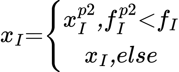 (20)
In the equation, 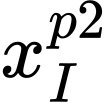 represents the new position that is to be calculated for the
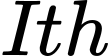 search agent, derived from the second phase of COA.
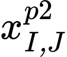 signifies its
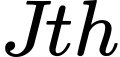 dimension, while
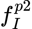 represents its objective function value. The decision to accept this position depends on a random number r in [0, 1], along with the iteration counter
 .
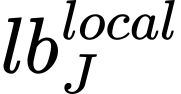 and
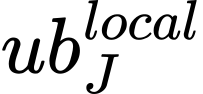 are the local lower and upper bounds for the
 decision variable, while
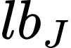 and
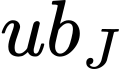 represent the global lower and upper bounds for the same variable.
(e ) Eddy Current Formation
In the marine ecosystem, the presence of eddies and Fish Aggregating Devices (FADs) significantly shapes the behavior of search agent. prey, for instance, tend to frequent the vicinity of FADs, dedicating the remainder of their time to extensive exploratory skips across different dimensions to locate areas with varying prey distributions. This interplay between FADs and extended skips effectively prevents the algorithm from becoming trapped in local optima, thereby enhancing its overall performance. The scenario involving FADs can be accurately represented within the algorithm’s modeling.

Here, the likelihood of FADs effect is represented as 𝐹𝐴𝐷𝑠, set at 0.2.  signifies a binary vector consisting of elements with values 0 and 1. 𝑟 stands for a uniformly distributed random number within the [0, 1] interval. Subscripts
 denote the indices referring to random numbers in the prey matrix.
(f) Memory updating
Search agent possess a remarkable memory that enables them to recall successful foraging locations. Similarly, the MPA retains the best solution achieved in prior iterations and assesses it against the current solution. If the current solution proves superior, it supplants the previous one, ensuring constant refinement in the optimization process.
Step 4. Determine the best solution. Return the so far acquired best solution.
Step 5. Terminate.
Save the so far best solution.
Three Layer Deep Learning for Physical rehabilitation
In this three-layer deep learning framework, the journey begins with feature extraction, optimizing the input data’s representation. Leveraging transfer learning augments this process. Next, the spotlight shifts to an attention-based Convolutional Neural Network that hones in on salient aspects of the feature set. The refined information then enters a Recurrent Neural Network (RNN) for sequential pattern analysis. Following this, two dense layers further process the data, and the network converges through fully connected layers. Ultimately, a Softmax layer provides predictive outcomes. This holistic approach, enriched by transfer learning and attention mechanisms, yields highly refined predictions.
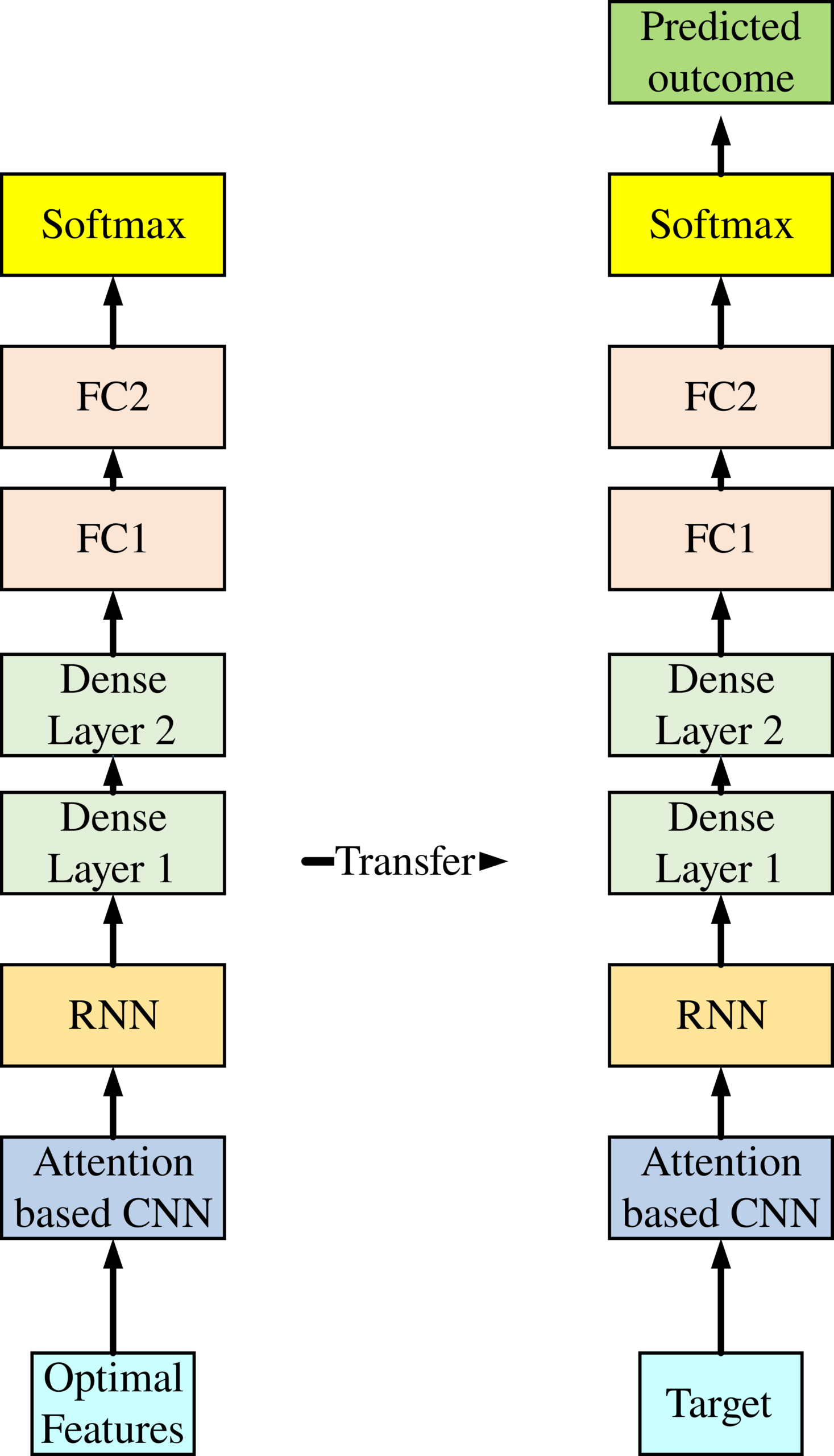
Figure : 3 Flow diagram of Three Layer deep learning
Optimized MLP
The Multi-Layer Perceptron, commonly referred to as MLP, comprises fully connected dense layers that can reshape input dimensions to the desired format. It’s a neural network with multiple layers where neurons are interconnected, allowing some neurons’ outputs to serve as inputs to others. An MLP typically features an input layer with one neuron per input, an output layer with neurons corresponding to desired outputs, and any number of hidden layers with varying node counts.
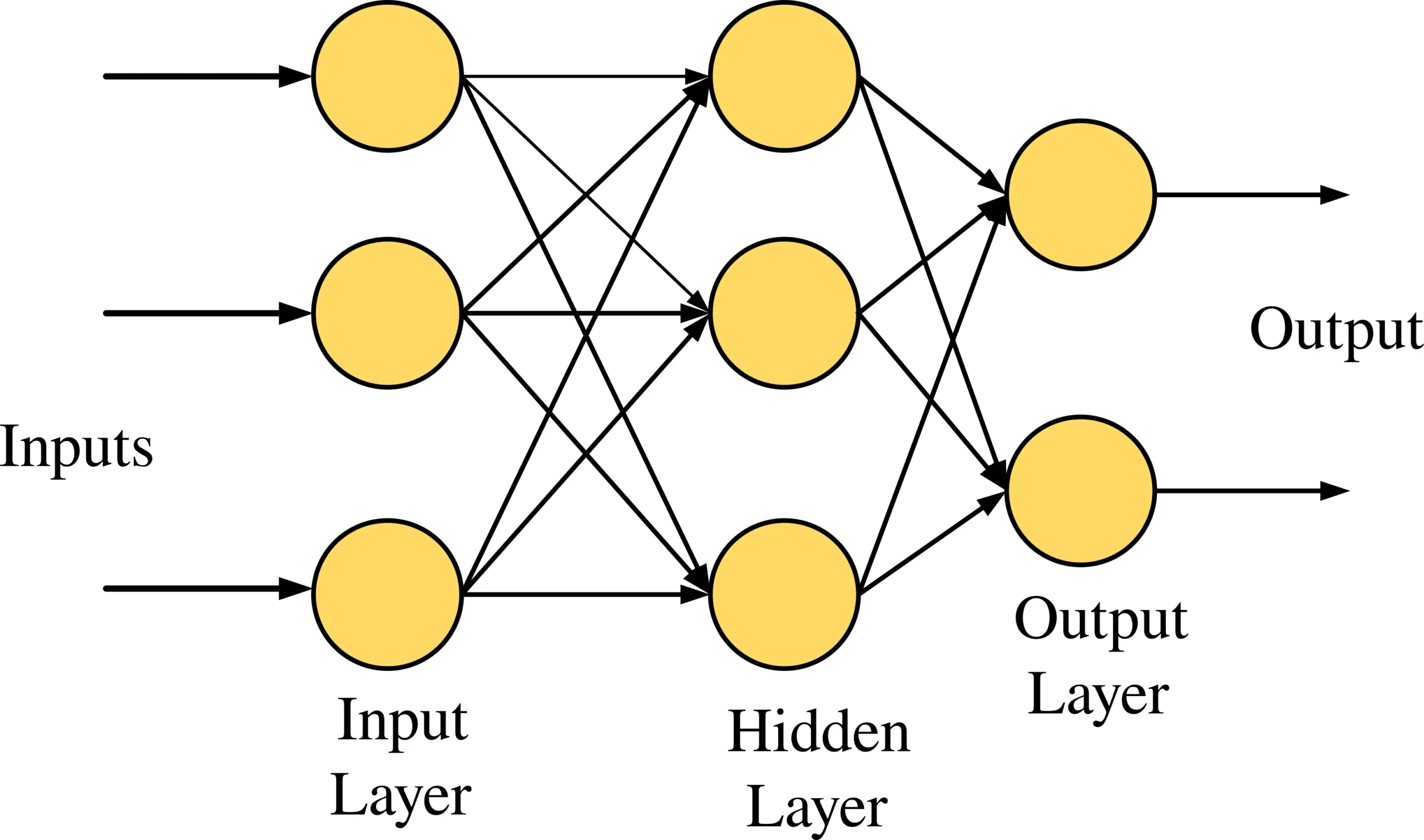
Figure 4: Optimized MLP
In the Fig 4., three input nodes correspond to three inputs, a hidden layer with three nodes, and an output layer with two nodes for two outputs. Information flows from input nodes to hidden layer nodes and then to output nodes. Each node employs a sigmoid activation function, converting real values to values between 0 and 1 via the sigmoid formula. To improve detection accuracy, the framework fine-tunes the hidden layers within the Multilayer Perceptron (MLP) using a novel hybrid optimization approach. This method combines traditional training techniques with advanced optimization strategies to enhance the model’s performance. By fine-tuning the hidden layers through this novel hybrid optimization model, the framework aims to improve the accuracy of the detection system.
Attention Based CNN
ABCNN as illustrated in Fig
5 uses an attention feature matrix denoted as  to influence its convolution process. The purpose of these attention features is to assign higher weights to those units in the left representation feature map
 that are relevant to units in the right representation feature map
 .
 Here, Unit can indicate individual words or phrases at various network levels.
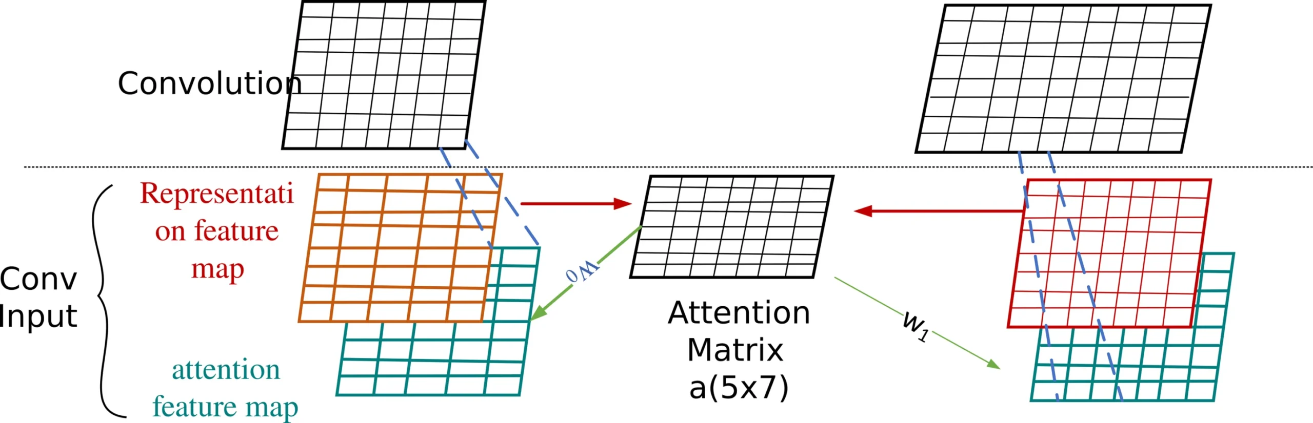
Figure 5: Block of ABCNN
This attention matrix A is generated by matching units in  with units in
 . The values in
 signify the attention distribution of each unit in
 concerning
 and vice versa.
 effectively serves as a novel feature map for both
 and
 . Each row or column corresponds to a feature vector of a unit in
 or
 . To harness this attention feature map optimally, it undergoes transformation into two blue matrices, aligning with the representation feature maps’ format. Consequently, the convolution operation takes input from both the original representation feature maps (in red) and the transformed attention-based feature maps (in green). This concept allows the attention feature map to guide convolution in learning counterpart-biased sentence representations, thereby enhancing the model’s capabilities.
Formally, for a sentence 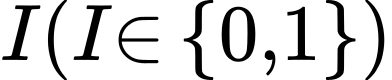 ), the representation feature map
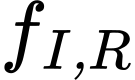 is created in
 ‘. The attention matrix
 is defined as follows in
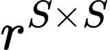 ‘.
 (29)
The match-score function can be defined using various methods, with a successful approach being  , where
 represents the Euclidean distance. Utilizing the attention matrix A, create the attention feature map
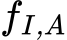 for
 as follows:
 (30)
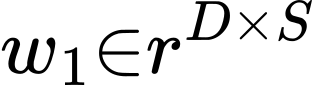
The model’s learnable parameters encompass weight matrices 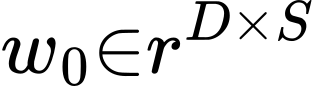 and
 . During training, the representation feature map
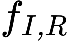 and the attention feature map
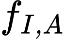 are combined into an order-3 tensor. This tensor undergoes convolution, yielding an elevated-level representation feature map for each
 . In Figure 4,
 comprises 5 units, and
 has 7. The convolution’s output, presented in the top layer with a filter width of
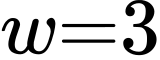 ,, results in a higher-level representation feature map with 7 columns for
 and 9 columns for

RNN
Unlike conventional feed-forward neural networks, recurrent neural networks are designed to handle sequential data, such as time-series or text. RNNs excel at processing continuous input spaces and generating sequence-to-sequence mappings. In an RNN, the input sequence  is processed sequentially, and the network maintains hidden states to capture temporal dependencies. This enables RNNs to produce an output sequence Y
 making them suitable for tasks like language modeling and translation. This fundamental distinction between RNNs and feed-forward networks highlights the versatility of RNNs in handling dynamic, sequential data.
 (31)
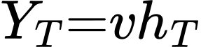 (32)
In the RNN architecture, comprising  and output
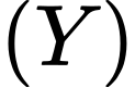 units, crucial parameters
 are learned through iterative loss minimization via backpropagation. RNNs are adept at processing variable-length inputs due to their dependency on these learned parameters, primarily
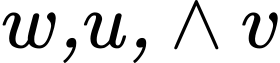 . However, challenges arise in training very deep RNNs, such as the risk of vanishing or exploding gradients. In applications like motion recognition, where continuous movement data is prevalent, RNNs prove suitable. The final hidden layer
 plays a role in determining motion labels, as it aggregates all relevant information. A feed-forward layer computes the probability matrix (as per Eq 32) for classification tasks, effectively mapping the input space to a fixed output space representing the number of classes.
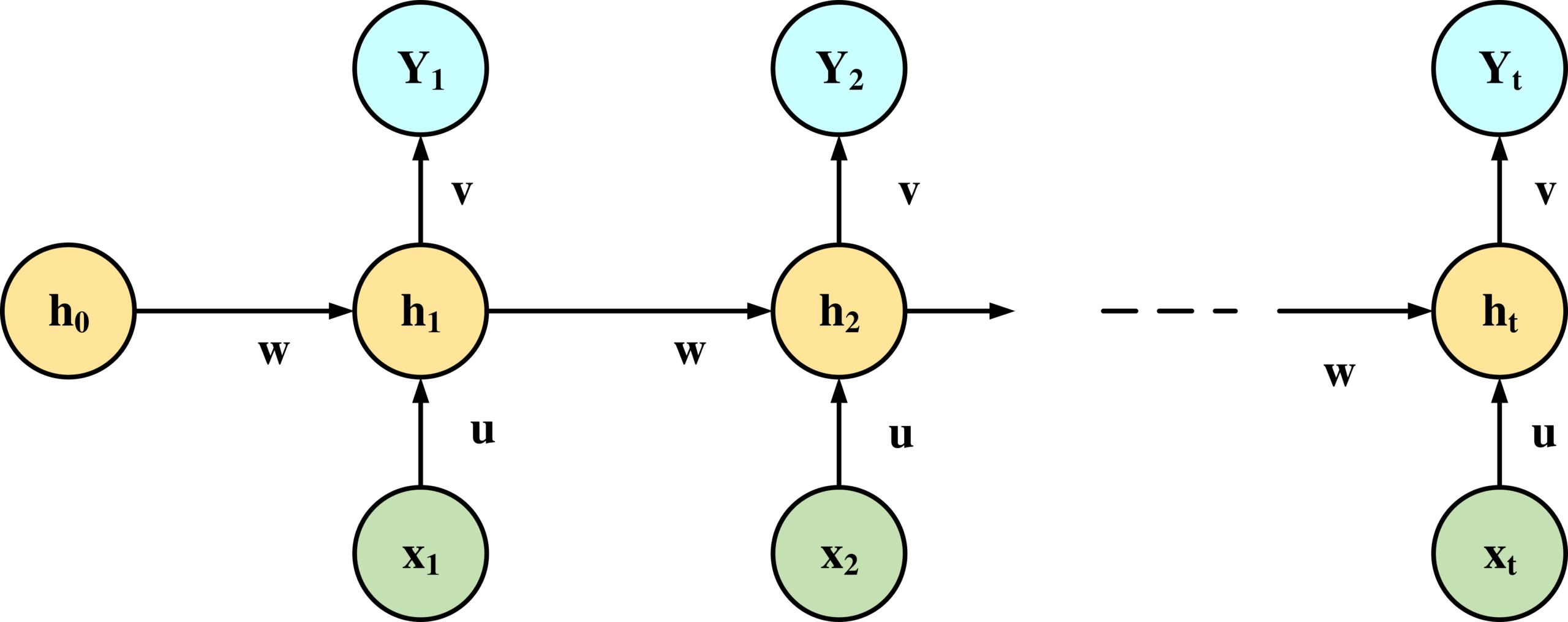
Figure 6: Architecture of RNN
Transfer Learning
Transfer learning for skeleton data is a approach that brings a new dimension to understanding and analyzing human or animal movements. In this context, skeletons represent the inferred or measured joint positions over time, often derived from images or sensor data. Transfer learning leverages the knowledge and features learned by a pretrained model on a related task and applies them to a different but closely connected problem. With data collection and preprocessing, ensuring data quality and consistency. A pretrained model, typically a deep neural network, is then chosen as a starting point. This model has already learned intricate patterns and hierarchical features from a vast dataset in its initial training, making it a valuable asset.
To adapt the model to the skeleton data, its architecture is adjusted. The final layers, originally designed for the pretrained task, are replaced or augmented with new layers capable of understanding the intricacies of skeleton input. For example, if the objective is human pose estimation, these layers may predict joint angles or key point positions. This transformation allows the model to gradually specialize in comprehending and interpreting the nuances of skeleton data. The heart of transfer learning lies in the transfer of knowledge. The modified model is initialized with the pretrained model’s weights, providing a head start in learning relevant information. Depending on the amount of data available for the target task, you can choose to freeze some layers (feature extraction) or fine-tune all layers for more task-specific learning. Training the model involves defining appropriate loss functions and utilizing optimization techniques to minimize them. Constant monitoring of the model’s performance on a validation dataset helps fine-tune hyperparameters for optimal results.
Transfer learning for skeleton data is invaluable when dealing with limited labeled data. It accelerates the learning process and often leads to models that excel in understanding and predicting skeletal structures and movements. This approach finds applications in diverse fields, including sports biomechanics, healthcare diagnostics, robotics, and more, where precise knowledge of skeletal movements is paramount for success.
Dense Layer
A dense layer, also known as a fully connected layer, serves as a cornerstone in neural networks, enabling the understanding of intricate data patterns and relationships. This layer connects every neuron to every neuron in the adjacent layers, facilitating comprehensive information exchange. Within this layer, each connection is associated with a weight, which is adjusted during training to learn from the data. Activation functions, like ReLU or sigmoid, introduce non-linearity, further enhancing the network’s ability to model intricate data relationships. Dense layers are critical for tasks such as natural language processing, image recognition and more, where they help capture and transform input data into meaningful predictions or classifications.
Fully Connected Layer
The fully connected layer, an integral component of neural networks, serves as a vital bridge for data transformation and abstraction. In this layer, every neuron is interconnected with all neurons in the preceding and succeeding layers, fostering extensive data interaction. Weighted connections between neurons adapt during training, permitting the network to grasp complex data patterns. By applying activation functions, such as ReLU or softmax, the fully connected layer introduces non-linearity, allowing the network to model intricate relationships in data. This layer plays a role in tasks like image recognition, natural language processing, and beyond, where it extracts crucial features, facilitating robust predictions and classifications.
Softmax
Softmax, a significant component in neural networks, is employed primarily for multi-class classification problems, where it transforms raw output scores into class probabilities. Its unique feature lies in its ability to normalize scores, ensuring that the probabilities sum up to 1. It accomplishes this by exponentiating the raw scores and then dividing them by the sum of all exponentiated scores. The result is a distribution where each class receives a probability score, Conveying the probability of input belonging to a particular class. Softmax plays a role in the decision-making process, determining the class with the highest probability. It finds extensive application in image classification, natural language processing, and various domains.
Visualization
Visualization method, built on the Grad-CAM technique, serves as a valuable complement to binary results by providing exercisers with detailed insights into incorrect body movements. Unlike traditional methods, this approach doesn’t rely on explicit templates. Instead, it autonomously learns comprehensive standards for correct movements from the dataset. By doing so, it offers a more holistic understanding of which body parts are deviating from the ideal form during exercise. This empowers users to make precise adjustments and improvements in their workout routines, enhancing the overall effectiveness of the system for fitness enthusiasts.
The Gradient-weighted Class Activation Mapping technique enhances the interpretability of CNN-based models by generating visual explanations. It elucidates the significance of input data concerning a specific target class. To create the class-discriminative localization map 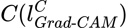 , the method calculates the gradient of the class c score
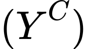 concerning the feature maps
 of a convolutional layer. These gradients are then globally average-pooled to derive neuron importance weights
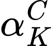 , which highlight the critical regions contributing to the classification decision for the class of interest. This process aids in understanding model behavior and its focus on specific features.
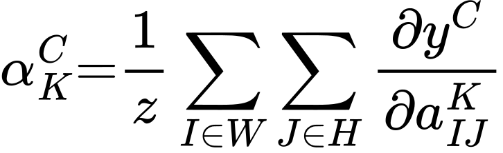 (33)
The Grad-CAM technique is represented by a forward activation maps weighted combination, followed by a ReLU , where the total number of pixels within the feature map is denoted as  . This formulation helps visualize and emphasize the regions contributing to the model’s decision for a specific class.
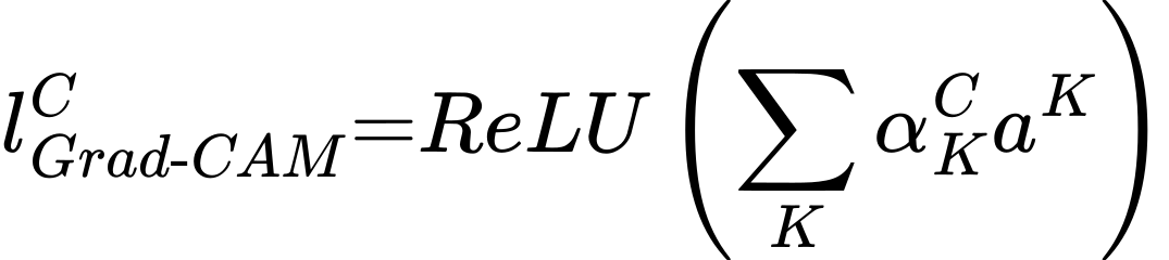 (34)
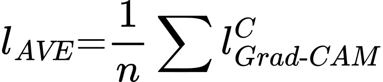
The resulting output, 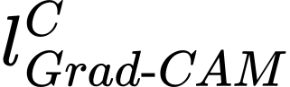 , serves as attention heat maps, revealing the specific areas that the neural networks prioritize. To discern distinctions in exercise classification, we employ Equation (35) to compute the average heat maps across all samples for each exercise category. This approach allows us to gain insights into how the model’s attention varies when distinguishing between different exercise categories, shedding light on the key visual cues and regions influencing the classification outcomes.
 (35)
Results and Discussion
Experimental Setup
In this research, to get the best accuracy the proposed model is implemented in Python with KIMORE dataset. Ex1, Ex2, Ex3, Ex4, Ex5 are the five types of Physical rehabilitation exercises in the KIMORE dataset. In Ex1, the individual grasps a bar, extending their arms alongside the body. In the first exercise, participants gradually raise their arms above their heads, keeping their elbows extended to stretch the trunk muscles. Their feet remain grounded, knees slightly bent, and they maintain a neutral pelvis position for form and effectiveness. Exercise 2 involves lifting the arms above the head with fully extended elbows while holding a bar with both hands (initial position). The participants gently tilt their trunk to the left and then to the right, ensuring it stays aligned with the frontal plane. They return to the initial position, focusing on avoiding backward or forward trunk bending. Feet are planted on the ground, slightly apart, with slightly flexed knees for stability. Exercise 3 focuses on trunk rotation. Beginning with arms extended at a 90-degree angle from the torso and fully extended elbows, participants gently rotate their torso first to the left and then to the right. After the rightward rotation, they return to the starting position while maintaining proper alignment without leaning forward or backward. Feet are firmly grounded, slightly apart, with knees slightly flexed for stability. In Exercise 4, individuals stand with their feet slightly apart and remain stationary. Without shifting their feet, they perform circular rotations of the pelvis, starting with clockwise rotations and then switching to counterclockwise rotations. This exercise enhances pelvis mobility within the transverse plane while maintaining a stable stance. Exercise 5 involves squatting. Beginning with arms aligned at a 90-degree angle to the trunk and fully extended elbows (initial position), participants bend their knees to approximately 60 to 70 degrees and then return to the starting position. Throughout, they must maintain proper alignment in the sagittal plane, preventing any forward or backward trunk bending.
Performance Comparison with Baseline Models
Table 2 presents the comprehensive performance metrics evaluation of the InceptionV3 model across five distinct exercises (Ex1 to Ex5). The accuracy of the model ranges from 0.859 to 0.93, with Ex2 achieving the highest accuracy at 0.93. Precision scores are consistently high, with Ex2 recording a precision of 0.95. Recall, sensitivity, and F1-score demonstrate the model’s ability to effectively identify relevant data points, with values mostly exceeding 0.9. Specificity and negative predictive value (NPV) showcase the model’s capability to accurately identify true negatives, with Ex5 achieving a specificity of 0.95. The Matthews Correlation Coefficient (MCC) reflects strong performance across all exercises, ranging from 0.82 to 0.905. False positive rate and false negative rate provide insights into model errors, with both typically around 0.09. Overall, the InceptionV3 model demonstrates robust performance across these exercises, with exercise-specific variations in metrics.
Table 2: Overall performance of the performance metrics of the model InceptionV3
| InceptionV3 | ||||
Metrics | Ex1 | Ex2 | Ex3 | Ex4 | Ex5 |
Accuracy | 0.901 | 0.93 | 0.901 | 0.859 | 0.9 |
Precision | 0.939 | 0.95 | 0.927 | 0.859 | 0.9 |
Recall | 0.901 | 0.9301 | 0.902 | 0.859 | 0.83 |
sensitivity | 0.901 | 0.9301 | 0.902 | 0.859 | 0.84 |
F1-score | 0.93 | 0.9301 | 0.92 | 0.859 | 0.9 |
Specificity | 0.939 | 0.9502 | 0.927 | 0.859 | 0.95 |
NPV | 0.903 | 0.9301 | 0.901 | 0.819 | 0.901 |
MCC | 0.905 | 0.93 | 0.902 | 0.82 | 0.89 |
FPR | 0.0791 | 0.0794 | 0.089 | 0.109 | 0.09 |
FNR | 0.079 | 0.0793 | 0.089 | 0.109 | 0.09 |
Table 3 provides an in-depth assessment of the ResNet model’s overall performance across five distinct exercises (Ex1 to Ex5). The model exhibits robust accuracy, with scores ranging from 0.852 to 0.955, with Ex1 achieving the highest accuracy at 0.955. Precision values consistently demonstrate the model’s capacity to produce precise positive predictions, with Ex2 recording the highest precision value of 0.961. Recall and sensitivity underscore the model’s proficiency in correctly identifying positive instances, with values mostly exceeding 0.85. F1-scores indicate strong model performance across exercises. Specificity and negative predictive value (NPV) highlight the model’s capacity to accurately identify true negatives, with Ex5 achieving an impressive specificity of 0.973. The Matthews Correlation Coefficient (MCC) signifies overall model effectiveness, ranging from 0.825 to 0.953. False positive rate and false negative rate illustrate the model’s errors, typically below 0.1. In summary, the ResNet model consistently delivers high performance across these exercises, with exercise-specific variations in metrics.
Table 3: Overall performance of the metrics of the Model ResNet
| Resnet | ||||
Metrics | Ex1 | Ex2 | Ex3 | Ex4 | Ex5 |
Accuracy | 0.955 | 0.953 | 0.931 | 0.852 | 0.913 |
Precision | 0.953 | 0.961 | 0.932 | 0.85 | 0.943 |
Recall | 0.955 | 0.951 | 0.933 | 0.852 | 0.863 |
sensitivity | 0.955 | 0.952 | 0.933 | 0.852 | 0.863 |
F1-score | 0.955 | 0.961 | 0.931 | 0.852 | 0.913 |
Specificity | 0.963 | 0.964 | 0.935 | 0.85 | 0.973 |
NPV | 0.925 | 0.952 | 0.931 | 0.832 | 0.913 |
MCC | 0.92 | 0.953 | 0.911 | 0.825 | 0.903 |
FPR | 0.0774 | 0.073 | 0.087 | 0.099 | 0.071 |
FNR | 0.0777 | 0.072 | 0.087 | 0.099 | 0.075 |
Table 4 offers a comprehensive evaluation of the Bi-LSTM model’s overall performance across five distinct exercises (Ex1 to Ex5). The model consistently displays strong accuracy, ranging from 0.87 to 0.96, with Ex2 achieving the highest accuracy at 0.96. Precision values indicate the ability of the model to correctly identify positive cases, with Ex2 and Ex3 recording the highest precision of 0.968 and 0.959, respectively. Recall and sensitivity underline the model’s ability to identify positive instances effectively, with values mainly exceeding 0.85. F1-scores reinforce strong model performance across exercises. Specificity and negative predictive value (NPV) underscore the model’s capacity to accurately identify true negatives, with Ex2 achieving an impressive specificity of 0.978. The Matthews Correlation Coefficient (MCC) reflects overall model effectiveness, ranging from 0.829 to 0.96. False positive rate and false negative rate showcase the model’s error rates, typically below 0.1. In summary, the Bi-LSTM model consistently exhibits robust performance across these exercises, with slight exercise-specific variations in metrics.
Table 4: Overall performance of the metrics of the model Bi-LSTM
| Bi-LSTM | ||||
Metrics | Ex1 | Ex2 | Ex3 | Ex4 | Ex5 |
Accuracy | 0.929 | 0.96 | 0.955 | 0.87 | 0.923 |
Precision | 0.959 | 0.968 | 0.959 | 0.88 | 0.953 |
Recall | 0.929 | 0.969 | 0.93 | 0.87 | 0.853 |
sensitivity | 0.929 | 0.969 | 0.93 | 0.87 | 0.853 |
F1-score | 00.959 | 00.96 | 00.955 | 00.87 | 00.923 |
Specificity | 00.959 | 00.978 | 00.959 | 00.88 | 00.963 |
NPV | 00.929 | 00.96 | 00.94 | 00.84 | 00.933 |
MCC | 00.925 | 00.96 | 00.92 | 00.829 | 00.903 |
FPR | 0.057 | 0.066 | 0.081 | 0.089 | 0.065 |
FNR | 0.067 | 0.06 | 0.081 | 0.089 | 0.065 |
Table 5 presents an overview of the comprehensive performance metrics for the LSTM[21] model across five different experiments (Ex1 to Ex5). The model showcases a consistent and noteworthy performance in these experiments. In terms of accuracy, LSTM[21] achieves high scores, ranging from 87% to 97%, demonstrating its ability to correctly classify data. The precision values for various experiments are impressive, fluctuating between 92% and 97%, signifying its accuracy in identifying positive instances. Moreover, the model consistently exhibits robust recall and sensitivity values, mostly above 87%, indicating its proficiency in capturing true positive instances. The F1-score, which balances precision and recall, maintains a strong presence at around 90% for most experiments. Specificity, the ability to identify true negatives, remains commendable, ranging from 86% to 98%. The Negative Predictive Value (NPV) stays above 84%, confirming the model’s aptitude for accurately predicting negative outcomes. The Matthews Correlation Coefficient (MCC) values are noteworthy, with scores ranging from 83% to 97%, highlighting the model’s overall strong performance. False Positive Rates and False Negative Rates are kept low, reinforcing the model’s reliability. In summary, LSTM[21] consistently demonstrates a high level of accuracy, precision, recall, specificity, and overall effectiveness across a range of experiments, making it a promising choice for classification tasks.
Table 5: Overall performance of the metrics of the model LSTM[21]
| LSTM[21] | ||||
Ex1 | Ex2 | Ex3 | Ex4 | Ex5 | |
Accuracy | 0.97 | 0.96 | 0.955 | 0.87 | 0.923 |
Precision | 0.967 | 0.97 | 0.955 | 0.92 | 0.97 |
Recall | 0.937 | 0.97 | 0.935 | 0.89 | 0.87 |
sensitivity | 0.937 | 0.97 | 0.935 | 0.89 | 0.87 |
F1-score | 00.957 | 00.97 | 00.945 | 00.9 | 00.91 |
Specificity | 00.977 | 00.97 | 00.979 | 00.86 | 00.98 |
NPV | 00.93 | 00.97 | 00.948 | 00.849 | 00.94 |
MCC | 00.93 | 00.965 | 00.93 | 00.83 | 00.9 |
FPR | 0.05 | 0.06 | 0.047 | 0.079 | 0.07 |
FNR | 0.057 | 0.05 | 0.077 | 0.085 | 0.05 |
Table 6 provides a comprehensive overview of the performance metrics for the CNN[14] model across five distinct experiments (Ex1 to Ex5). The CNN[14] model consistently demonstrates robust performance in these experiments, showcasing its effectiveness in various classification tasks.In terms of accuracy, CNN[14] consistently achieves high scores, ranging from 90% to 98%, underscoring its proficiency in correctly classifying data. Precision values across experiments are notably high, fluctuating between 93% and 99%, emphasizing its accuracy in correctly identifying positive instances. The model consistently exhibits strong recall and sensitivity values, predominantly above 88%, indicating its ability to capture true positive instances effectively. The F1-score, which balances recall and precision , maintains a strong presence at around 91% for most experiments. Specificity, measuring the model’s ability to identify true negatives, remains commendable, ranging from 87% to 99%. The Negative Predictive Value (NPV) generally stays above 85%, affirming the model’s capability to predict negative outcomes accurately. The Matthews Correlation Coefficient (MCC) values are substantial, with scores ranging from 83% to 97%, highlighting the model’s overall strong performance. False Positive Rates and False Negative Rates are consistently low, further affirming the model’s reliability and robustness. In summary, CNN[14] consistently demonstrates high levels of accuracy, precision, recall, specificity, and overall effectiveness across a range of experiments, establishing its merit as a dependable choice for classification tasks.
Table 6: Overall performance of the metrics of model CNN[14]
CNN[14] | |||||
Metrics | Ex1 | Ex2 | Ex3 | Ex4 | Ex5 |
Accuracy | 0.969 | 0.98 | 0.965 | 0.9 | 0.95 |
Precision | 0.979 | 0.99 | 0.975 | 0.93 | 0.98 |
Recall | 0.949 | 0.99 | 0.945 | 0.9 | 0.88 |
sensitivity | 0.949 | 0.99 | 0.945 | 0.9 | 0.88 |
F1-score | 00.969 | 00.99 | 00.965 | 00.91 | 00.92 |
Specificity | 00.989 | 00.99 | 00.975 | 00.87 | 00.99 |
NPV | 00.933 | 00.996 | 00.95 | 00.85 | 00.95 |
MCC | 00.939 | 00.97 | 00.941 | 00.832 | 00.913 |
FPR | 0.037 | 0.03 | 0.02 | 0.063 | 0.06 |
FNR | 0.049 | 0.03 | 0.06 | 0.083 | 0.03 |
Table 7 offers a comprehensive view of the performance metrics for the proposed model across five distinct experiments (Ex1 to Ex5). The proposed model Coati Predator Optimization Algorithm consistently demonstrates exceptional performance, underlining its effectiveness in diverse classification tasks. In terms of accuracy, the proposed model achieves consistently high scores, ranging from 90.4% to a perfect 100%, illustrating its remarkable ability to correctly classify data. Precision values are consistently at or near 100%, showcasing its precision in correctly identifying positive instances. The model consistently maintains robust recall and sensitivity values, primarily above 89%, signifying its skill in capturing true positive instances effectively. The F1-score, a balance between precision and recall, remains notably high, around 93%, for most experiments. Specificity, measuring the model’s ability to identify true negatives, is impressive, reaching perfection in some experiments. The Negative Predictive Value (NPV) stays above 85%, confirming the model’s proficiency in accurately predicting negative outcomes. The Matthews Correlation Coefficient (MCC) values are substantial, with scores consistently above 84%, highlighting the model’s overall exceptional performance. False Positive Rates and False Negative Rates are consistently low, further emphasizing the model’s reliability and robustness. In summary, the proposed model consistently exhibits outstanding levels of accuracy, precision, recall, specificity, and overall effectiveness across various experiments, establishing its excellence as a dependable choice for classification tasks.
Table 7: overall performance of the metrics of the proposed model (CPOA)
| Proposed (CPOA) | ||||
| Ex1 | Ex2 | Ex3 | Ex4 | Ex5 |
Accuracy | 0.972 | 1 | 0.975 | 0.904 | 0.966 |
Precision | 1 | 1 | 1 | 0.952 | 1 |
Recall | 0.952 | 1 | 0.95 | 0.909 | 0.894 |
sensitivity | 0.952 | 1 | 0.95 | 0.909 | 0.894 |
F1-score | 0.975 | 1 | 0.974 | 0.9302 | 0.944 |
Specificity | 1 | 1 | 1 | 0.894 | 1 |
NPV | 0.939 | 1 | 0.952 | 0.859 | 0.952 |
MCC | 0.945 | 1 | 0.951 | 0.842 | 0.923 |
FPR | 0.01 | 0.01 | 0.01 | 0.05 | 0.05 |
FNR | 0.047 | 0.01 | 0.05 | 0.08 | 0.02 |
|
|
(a ) | (b) |
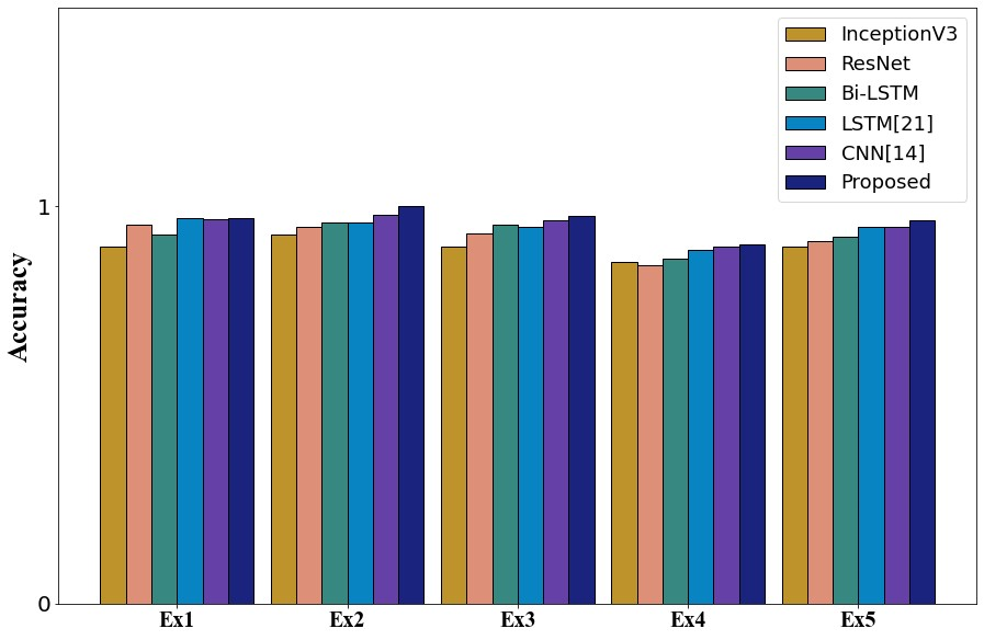
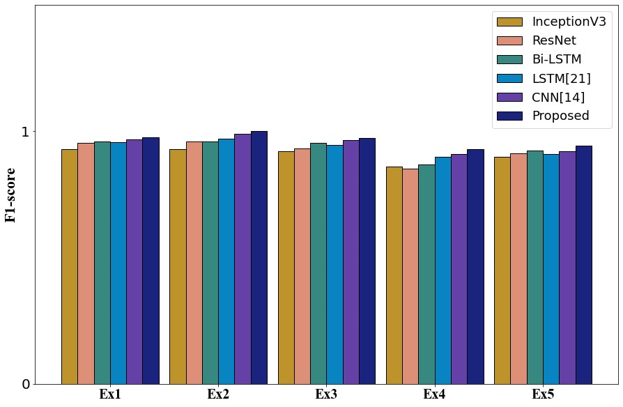
Figure 7: Graphical format of the performance metrics –(a) Accuracy (b) F1-Score of the models
Figure 7 compares accuracy in panel (a) and F1-score in panel (b) across Ex1–Ex5 for the proposed model and the baseline models.
|
|
(a) | (b) |
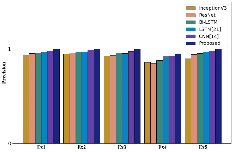
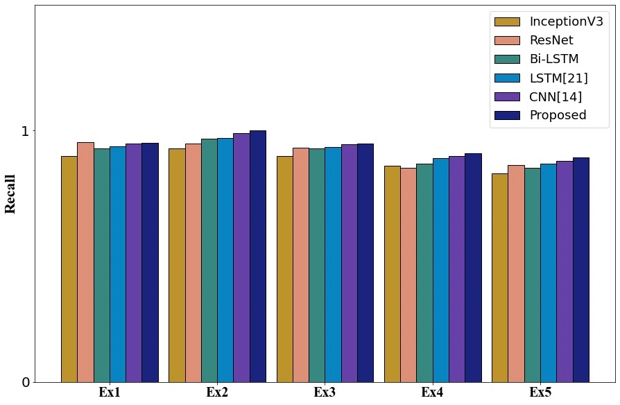
Figure 8: Graphical format of the performance metrics- (a) Precision (b) Recall of the models
Figure 8 compares precision in panel (a) and recall in panel (b) across Ex1–Ex5. The bars show the reported results for the proposed model and the baseline models.
|
|
(a) | (b) |
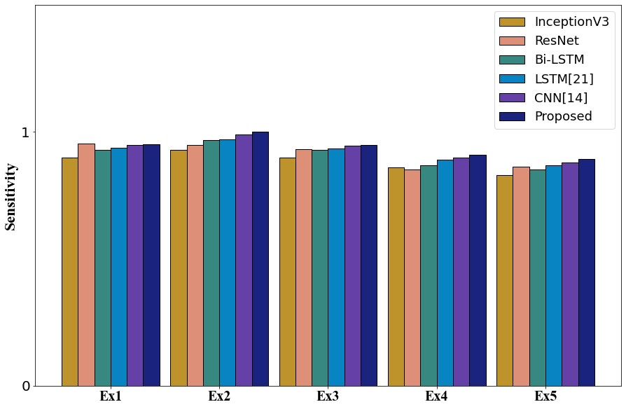
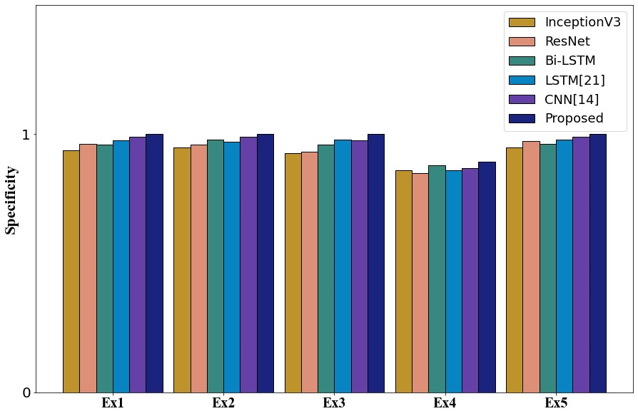
Figure 9: Graphical format of the performance metrics- (a) Sensitivity (b) Specificity of the models
Figure 9 compares sensitivity in panel (a) and specificity in panel (b) across the five exercises.
|
|
(a) | (b) |
|
|
(c ) | (d) |
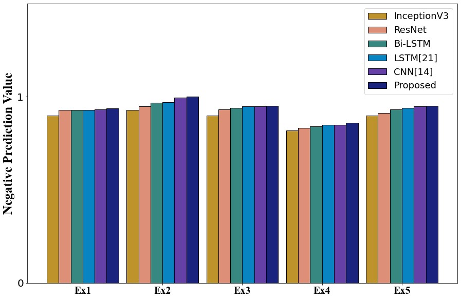
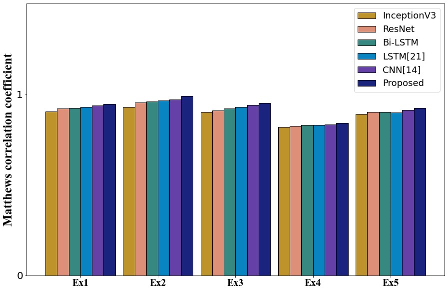
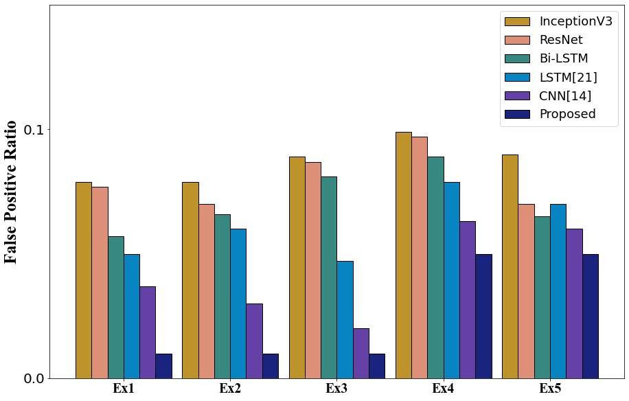
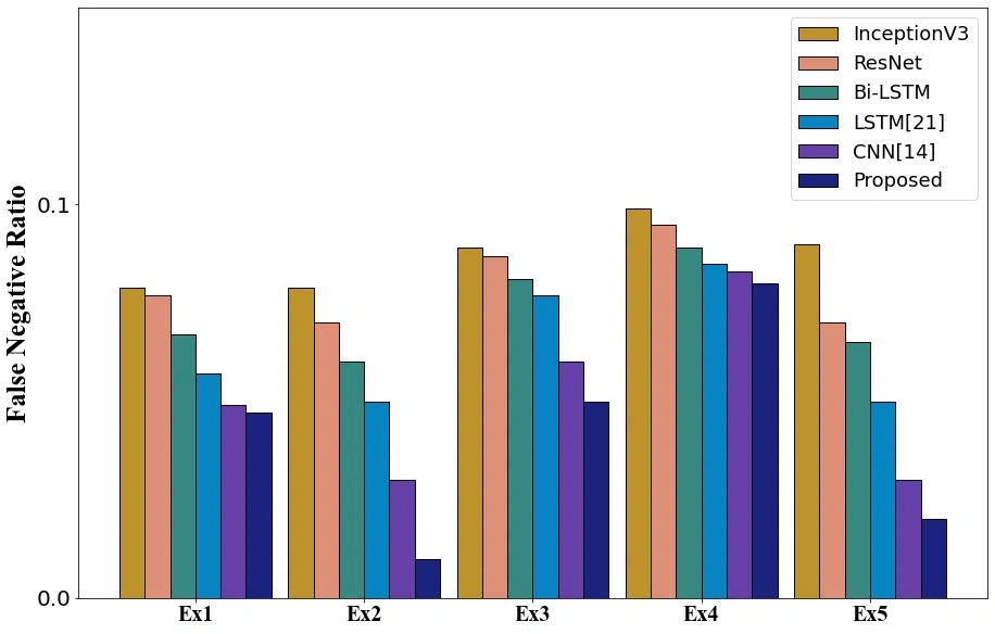
Figure 10: Graphical format of the performance metrics- (a) NPV (b) MCC (c ) FPR (d) FNR for the models
Figure 10 compares negative predictive value (a), Matthews correlation coefficient (b), false positive rate (c) and false negative rate (d) for the proposed model and the baseline models across Ex1–Ex5.
Conclusion
This study develops a computational framework for multimodal human movement assessment. Skeleton-data preprocessing, GAN-based augmentation and CLAHE prepare the input material for analysis. Joint-level, limb-level, temporal and statistical descriptors represent different aspects of movement. The proposed Coati Predator Optimization Algorithm combines Coati Optimization and Marine Predators Optimization for feature selection and model tuning. The learning framework includes an optimized MLP, an attention-based CNN and an RNN, with transfer learning, while Grad-CAM provides visual explanations of model outputs. The manuscript reports comparisons across five KIMORE exercise categories using classification metrics and graphical results. Implemented in Python, the framework connects movement representation, hybrid optimisation and neural modelling within one assessment pipeline.
References
Amatriain-Fernández, S., Murillo-Rodríguez, E.S., Gronwald, T., Machado, S. and Budde, H., 2020. Benefits of physical activity and physical exercise in the time of pandemic. Psychological Trauma: Theory, Research, Practice, and Policy, 12(S1), p.S264.
Deb, S., Islam, M.F., Rahman, S. and Rahman, S., 2022. Graph convolutional networks for assessment of physical rehabilitation exercises. IEEE Transactions on Neural Systems and Rehabilitation Engineering, 30, pp.410-419.
Yu, X. and Xiong, S., 2019. A dynamic time warping based algorithm to evaluate kinect-enabled home-based physical rehabilitation exercises for older people. Sensors, 19(13), p.2882.
Zhang, W., Su, C. and He, C., 2020. Rehabilitation exercise recognition and evaluation based on smart sensors with deep learning framework. IEEE Access, 8, pp.77561-77571.
Wu, N.N., Tian, H., Chen, P., Wang, D., Ren, J. and Zhang, Y., 2019. Physical exercise and selective autophagy: benefit and risk on cardiovascular health. Cells, 8(11), p.1436.
Semwal, V., Singh, G., Crespo, U. and González, R., 2021. Heterogeneous Computing Model for Post-injury Walking Pattern restoration and Postural Stability Rehabilitation Exercise Recognition.
Capecci, M., Ceravolo, M.G., Ferracuti, F., Iarlori, S., Monteriu, A., Romeo, L. and Verdini, F., 2019. The KIMORE dataset: KInematic assessment of MOvement and clinical scores for remote monitoring of physical REhabilitation. IEEE Transactions on Neural Systems and Rehabilitation Engineering, 27(7), pp.1436-1448.
Baltzer W I, Smithostrin S, Warnock J J, et al. Evaluation of the clinical effects of diet and physical rehabilitation in dogs following tibial plateau leveling osteotomy[J]. Journal of the American Veterinary Medical Association, 2018, 252(6):686-700.
Rochester, C.L., 2019. Patient assessment and selection for pulmonary rehabilitation. Respirology, 24(9), pp.844-853.
Jiang, Y., 2020. Combination of wearable sensors and internet of things and its application in sports rehabilitation. Computer Communications, 150, pp.167-176.
Kitzman, D.W., Whellan, D.J., Duncan, P., Pastva, A.M., Mentz, R.J., Reeves, G.R., Nelson, M.B., Chen, H., Upadhya, B., Reed, S.D. and Espeland, M.A., 2021. Physical rehabilitation for older patients hospitalized for heart failure. New England Journal of Medicine, 385(3), pp.203-216.
Fossati, C., Torre, G., Vasta, S., Giombini, A., Quaranta, F., Papalia, R. and Pigozzi, F., 2021. Physical exercise and mental health: The routes of a reciprocal relation. International Journal of Environmental Research and Public Health, 18(23), p.12364.
Zhu, Z. A., Lu, Y. C., You, C. H., & Chiang, C. K. (2019). Deep learning forsensor-based rehabilitation exercise recognition and evaluation. Sensors, 19(4),887.
Panwar, M., Biswas, D., Bajaj, H., Jöbges, M., Turk, R., Maharatna, K. and Acharyya, A., 2019. Rehab-net: Deep learning framework for arm movement classification using wearable sensors for stroke rehabilitation. IEEE Transactions on Biomedical Engineering, 66(11), pp.3026-3037.
Sun, M., Zhao, S., Gilvary, C., Elemento, O., Zhou, J. and Wang, F., 2020. Graph convolutional networks for computational drug development and discovery. Briefings in bioinformatics, 21(3), pp.919-935.
Liao, Y., Vakanski, A. and Xian, M., 2020. A deep learning framework for assessing physical rehabilitation exercises. IEEE Transactions on Neural Systems and Rehabilitation Engineering, 28(2), pp.468-477.
Kanade, A., Sharma, M. and Muniyandi, M., 2022. A Robust and Scalable Attention Guided Deep Learning Framework for Movement Quality Assessment. arXiv preprint arXiv:2204.07840.
Capecci, M., Ceravolo, M.G., Ferracuti, F., Iarlori, S., Kyrki, V., Monteriu, A., Romeo, L. and Verdini, F., 2018. A Hidden Semi-Markov Model based approach for rehabilitation exercise assessment. Journal of biomedical informatics, 78, pp.1-11.
Caru, M., Curnier, D., Bousquet, M. and Kern, L., 2020. Evolution of depression during rehabilitation program in patients with cardiovascular diseases. Disability and Rehabilitation, 42(3), pp.378-384.
Mandolesi, L., Polverino, A., Montuori, S., Foti, F., Ferraioli, G., Sorrentino, P. and Sorrentino, G., 2018. Effects of physical exercise on cognitive functioning and wellbeing: biological and psychological benefits. Frontiers in psychology, p.509.
Rahman, Z.U., Ullah, S.I., Salam, A., Rahman, T., Khan, I. and Niazi, B., 2022. Automated detection of rehabilitation exercise by stroke patients using 3-layer CNN-LSTM model. Journal of Healthcare Engineering, 2022.
Schez-Sobrino, S., Vallejo, D., Monekosso, D.N., Glez-Morcillo, C. and Remagnino, P., 2020. A distributed gamified system based on automatic assessment of physical exercises to promote remote physical rehabilitation. IEEE Access, 8, pp.91424-91434.
Iwao, Y., Shigeishi, H., Takahashi, S., Uchida, S., Kawano, S. and Sugiyama, M., 2019. Improvement of physical and oral function in community‐dwelling older people after a 3‐month long‐term care prevention program including physical exercise, oral health instruction, and nutritional guidance. Clinical and Experimental Dental Research, 5(6), pp.611-619.
Whyte, J., Dijkers, M.P., Fasoli, S.E., Ferraro, M., Katz, L.W., Norton, S., Parent, E., Pinto, S.M., Sisto, S.A., Van Stan, J.H. and Wengerd, L., 2021. Recommendations for reporting on rehabilitation interventions. American Journal of Physical Medicine & Rehabilitation, 100(1), pp.5-16.
van der Windt, D.J., Sud, V., Zhang, H., Tsung, A. and Huang, H., 2018. The effects of physical exercise on fatty liver disease. Gene expression, 18(2), p.89.
Cite This Work
To export a reference to this article please select a referencing stye below:

Academic Master Education Team is a group of academic editors and subject specialists responsible for producing structured, research-backed essays across multiple disciplines. Each article is developed following Academic Master’s Editorial Policy and supported by credible academic references. The team ensures clarity, citation accuracy, and adherence to ethical academic writing standards
Content reviewed under Academic Master Editorial Policy.