
 Civil Engineering
Textbook
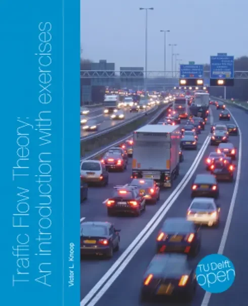
Traffic Flow Theory: An introduction with exercises
Not rated yetRate this bookTraffic Flow Theory: An Introduction with Exercises explains road traffic through complementary microscopic and macroscopic descriptions. Victor L. Knoop develops measurements, cumulative curves, flow-density relationships, shock waves, driver behavior, network models, and alternative mathematical representations. The complete third-edition PDF contains fifteen chapters, followed by exercise solutions and supporting material. This guide keeps that full sequence rather than stopping at the introductory fundamental diagram. Its recurring concern is connecting a mathematical description with what vehicles, queues, and traffic states actually do. Readers benefit from calculus, basic statistics, and careful attention to units and conservation.
Read on the publisher’s website. Opens in a new tab.
 Free
About this book
Overview
Traffic Flow Theory: An Introduction with Exercises explains road traffic through complementary microscopic and macroscopic descriptions. Victor L. Knoop develops measurements, cumulative curves, flow-density relationships, shock waves, driver behavior, network models, and alternative mathematical representations. The complete third-edition PDF contains fifteen chapters, followed by exercise solutions and supporting material. This guide keeps that full sequence rather than stopping at the introductory fundamental diagram. Its recurring concern is connecting a mathematical description with what vehicles, queues, and traffic states actually do. Readers benefit from calculus, basic statistics, and careful attention to units and conservation.
How to study this book
Draw a space-time diagram before solving a queue or shock-wave problem. State whether a quantity describes an individual vehicle, a road location, a time interval, or an area of space-time. Check the units of flow, density, speed, headway, and accumulation at every step. Solve exercises before reading the source solutions and compare reasoning as well as the final number. When moving between microscopic and macroscopic descriptions, explain what information is averaged away. For simulations, define the boundary conditions and compare outputs with conservation and plausible behavior before interpreting an attractive plot.
Chapter and section study guide
Chapter 1 — Variables
Traffic variables change meaning with the level and method of observation. Microscopic descriptions follow vehicles, while macroscopic descriptions summarize many vehicles through quantities such as flow, density, and speed. Local, instantaneous, and space-time measurements do not automatically produce interchangeable averages. Stationarity and homogeneity simplify analysis but should be stated rather than silently assumed. The chapter establishes a vocabulary for later models and guards against dimensional mistakes. Interpret a measured quantity by identifying where, when, and over which vehicles it was obtained.
Study application: Specify how you would measure flow, density, and speed on a road segment and explain why the chosen averaging method matters.
Chapter 2 — Cumulative Curves
Cumulative arrival and departure curves count vehicles over time and reveal queues, travel times, and delays through their geometric relationships. Slopes represent rates, vertical separations can represent accumulation, and horizontal separations can represent time differences under appropriate matching assumptions. The method connects a conservation account with a visual description of congestion. A curve must remain consistent with counting order and the system boundary. Distinguish queue length in vehicles from physical queue length along a road; converting between them requires additional spatial information.
Study application: Construct arrival and departure curves for a short capacity restriction and identify maximum accumulation and one vehicle’s delay.
Chapter 3 — Relationships of Traffic Variables
Relations among flow, density, and speed organize the transition from free-flowing to congested conditions. The fundamental diagram is a model or empirical relationship, not a universal curve independent of road and measurement conditions. Capacity, critical density, and congested states acquire meaning within that description. Different data aggregation methods and changing conditions can alter observed patterns. Study the assumptions behind a selected curve before using it to infer an unmeasured variable. The chapter prepares the state descriptions used in shock-wave and dynamic traffic models.
Study application: Plot a simple fundamental diagram, label its regimes, and explain why the same flow can be associated with different traffic states.
Chapter 4 — Shock Wave Theory
A shock separates traffic states with different density and flow, and its propagation follows conservation. The wave speed depends on changes between states rather than the speed of an individual vehicle. Queues can therefore move upstream while all vehicles continue downstream. Space-time diagrams make interactions between fronts visible and help locate queue growth and dissipation. The chapter requires consistent sign conventions and state definitions. Before calculating, identify the states on each side of a front and check whether the resulting motion is physically plausible.
Study application: Use two traffic states to compute a shock speed and draw vehicle trajectories crossing the moving boundary.
Chapter 5 — Shockwave Theory: Moving Bottlenecks
A slow-moving vehicle or restriction creates a bottleneck whose position changes with time. Its interaction with surrounding traffic differs from that of a fixed capacity reduction. Analyze flows relative to the moving boundary and identify the traffic states that can pass or accumulate behind it. The chapter extends shock-wave reasoning while retaining vehicle conservation. A moving bottleneck may produce several fronts and changing queue geometry. Explain the mechanism in a space-time diagram before relying on an equation that obscures which reference frame is being used.
Study application: Compare a fixed restriction and a moving slow vehicle under the same demand, marking the bottleneck trajectory and queue boundaries.
Chapter 6 — Traffic States and Phenomena
Observed traffic includes free flow, congestion, breakdown, queue discharge, and transitions that challenge an overly simple equilibrium picture. Capacity and throughput can depend on state and history rather than a single permanent number. The chapter connects empirical phenomena with the models used to explain them. Distinguish a recurring observation from an assumption introduced for analytical convenience. When data appear inconsistent with a fundamental diagram, investigate measurement, nonstationarity, and interactions before discarding the evidence. Model selection should follow the phenomenon being studied.
Study application: Describe a traffic breakdown using demand, bottleneck supply, observed states, and the limitations of a stationary equilibrium explanation.
Chapter 7 — Car-following
Car-following models describe how a driver responds to a leading vehicle, often through spacing, relative speed, desired speed, and reaction. Different formulations encode different behavioral assumptions and can produce different stability properties. A reasonable equilibrium gap does not guarantee realistic transient behavior. Calibration and validation require appropriate trajectory data and attention to the conditions being represented. Connect parameters with behavior rather than treating them as arbitrary numerical knobs. Study how a small disturbance can decay or grow as it passes through a line of vehicles.
Study application: Sketch a leader’s braking event and explain which observations would help distinguish two proposed follower-response models.
Chapter 8 — Microscopic Lane Change Models
Lane changes involve motivation, opportunities, safety conditions, and interactions with surrounding vehicles. Mandatory changes near an exit differ from discretionary changes intended to improve progress. A model must represent both the decision and its effects on the target and original lanes. Simplified rules can create unrealistic behavior if incentives and gap acceptance are disconnected. The chapter complements longitudinal car-following with lateral decisions. Evaluate whether a lane-change model reproduces the phenomenon of interest rather than assuming more detailed rules always produce more useful predictions.
Study application: Identify incentive and safety conditions for a hypothetical merge and trace its effects on vehicles in both lanes.
Chapter 9 — Use of Traffic Models
Traffic models support explanation, assessment, and decision-making, but usefulness depends on the question and available evidence. Microscopic and macroscopic approaches trade detail, data demands, computation, and interpretability. Calibration fits parameters, while validation assesses performance on evidence not simply reused for fitting. Boundary conditions, demand assumptions, and measurement uncertainty can dominate results. The chapter encourages a disciplined modeling workflow instead of treating a simulation as an automatic forecast. State the intended use and acceptance criteria before selecting software or increasing model complexity.
Study application: Write a short model-selection brief for a bottleneck study, including purpose, data, calibration, validation, and limitations.
Chapter 10 — Macroscopic Dynamic Traffic Flow Models
Macroscopic dynamic models combine conservation with relationships describing how traffic moves through space and time. They represent evolving density and flow rather than isolated equilibrium points. Discretization introduces numerical choices that must preserve plausible propagation and vehicle counts. Demand and supply at boundaries determine which flows can actually occur. The chapter connects continuum reasoning with implementable models and highlights the meaning of assumptions. A simulation result should be checked against conservation and known limiting cases before it is used to compare management strategies.
Study application: Describe how a capacity drop enters a macroscopic model and identify conservation checks for its numerical output.
Chapter 11 — An Introduction to Node Models
Road networks require rules at merges, diverges, and intersections as well as models for links. Node models distribute feasible flows according to sending demand, receiving capacity, turning movements, and priorities. A locally plausible link model can still produce unrealistic network behavior if junction rules violate constraints. The chapter introduces the logic needed to connect roads consistently. Distinguish desired movements from flows that downstream conditions permit. Spillback makes these interactions important because congestion in one part of a network can restrict apparently separate movements.
Study application: Analyze a merge with two incoming links and a constrained downstream link, stating feasibility limits and a transparent allocation rule.
Chapter 12 — Macroscopic Fundamental Diagram
A network-level relation between accumulation and production summarizes traffic across an area. Aggregation can support management insights but may conceal uneven congestion and route differences. The chapter explains why a network relationship is not simply a single-road fundamental diagram scaled upward. Heterogeneity, measurement boundaries, and loading history influence the observed pattern. Interpret accumulation and production with their proper units and spatial coverage. Network management questions should consider whether the aggregated state captures the conditions that actually constrain movement.
Study application: Compare two networks with equal vehicle accumulation but different spatial congestion patterns and explain why their production could differ.
Chapter 13 — Method of Characteristics
Characteristics describe how information associated with traffic states propagates through a conservation model. They help connect the mathematical equation with the motion of disturbances in space-time. Smooth regions and shocks require different treatment, and intersecting characteristics signal where a simple smooth description fails. The chapter provides a more analytical view of dynamics previously represented through state diagrams and numerical models. Distinguish characteristic speed from vehicle speed and shock speed. A clear diagram often reveals the structure of a solution before a full calculation is attempted.
Study application: Draw characteristic lines for a simple initial traffic condition and explain where a discontinuity may need separate conservation treatment.
Chapter 14 — Headway Models
Headways describe spacing in time between vehicles and provide a probabilistic perspective on arrivals and interactions. A distribution must fit the mechanism and constraints of the setting; independent arrivals differ from closely following platoons. Mean headway alone does not describe variability or the likelihood of a usable gap. The chapter connects statistical descriptions with practical questions such as gap acceptance and flow. Check whether observations satisfy the assumptions of a chosen distribution before interpreting its parameters. Distinguish a model for free arrivals from one for constrained following behavior.
Study application: Compare two headway distributions with the same mean and explain how their differences could affect opportunities to cross or merge.
Chapter 15 — Traffic State Dynamics in Three Representations
The final chapter relates alternative representations of traffic dynamics and shows how the same process can be described using different variables and coordinates. Changing representation can simplify a particular problem but also changes what is directly observed or calculated. Consistency requires tracking how vehicle labels, time, location, spacing, and density relate. This synthesis connects earlier microscopic, cumulative, and macroscopic perspectives. The goal is not to memorize separate formulas but to understand their shared conservation structure and the circumstances in which one description is more convenient.
Study application: Represent a small queueing example in three compatible ways and explain which quantities are easiest to read in each.
Reflection and review
- How can a queue move upstream while vehicles move downstream?
- Which information is lost when individual trajectories are aggregated into a network measure?
- What evidence would show that a model fits data yet fails its intended decision purpose?
Source and edition notes
Third edition, November 2020; fifteen chapters, 267 PDF pages.
Book summary
Overview
Traffic Flow Theory: An Introduction with Exercises explains road traffic through complementary microscopic and macroscopic descriptions. Victor L. Knoop develops measurements, cumulative curves, flow-density relationships, shock waves, driver behavior, network models, and alternative mathematical representations. The complete third-edition PDF contains fifteen chapters, followed by exercise solutions and supporting material. This guide keeps that full sequence rather than stopping at the introductory fundamental diagram. Its recurring concern is connecting a mathematical description with what vehicles, queues, and traffic states actually do. Readers benefit from calculus, basic statistics, and careful attention to units and conservation.
How to study this book
Draw a space-time diagram before solving a queue or shock-wave problem. State whether a quantity describes an individual vehicle, a road location, a time interval, or an area of space-time. Check the units of flow, density, speed, headway, and accumulation at every step. Solve exercises before reading the source solutions and compare reasoning as well as the final number. When moving between microscopic and macroscopic descriptions, explain what information is averaged away. For simulations, define the boundary conditions and compare outputs with conservation and plausible behavior before interpreting an attractive plot.
Chapter and section study guide
Chapter 1 — Variables
Traffic variables change meaning with the level and method of observation. Microscopic descriptions follow vehicles, while macroscopic descriptions summarize many vehicles through quantities such as flow, density, and speed. Local, instantaneous, and space-time measurements do not automatically produce interchangeable averages. Stationarity and homogeneity simplify analysis but should be stated rather than silently assumed. The chapter establishes a vocabulary for later models and guards against dimensional mistakes. Interpret a measured quantity by identifying where, when, and over which vehicles it was obtained.
Study application: Specify how you would measure flow, density, and speed on a road segment and explain why the chosen averaging method matters.
Chapter 2 — Cumulative Curves
Cumulative arrival and departure curves count vehicles over time and reveal queues, travel times, and delays through their geometric relationships. Slopes represent rates, vertical separations can represent accumulation, and horizontal separations can represent time differences under appropriate matching assumptions. The method connects a conservation account with a visual description of congestion. A curve must remain consistent with counting order and the system boundary. Distinguish queue length in vehicles from physical queue length along a road; converting between them requires additional spatial information.
Study application: Construct arrival and departure curves for a short capacity restriction and identify maximum accumulation and one vehicle’s delay.
Chapter 3 — Relationships of Traffic Variables
Relations among flow, density, and speed organize the transition from free-flowing to congested conditions. The fundamental diagram is a model or empirical relationship, not a universal curve independent of road and measurement conditions. Capacity, critical density, and congested states acquire meaning within that description. Different data aggregation methods and changing conditions can alter observed patterns. Study the assumptions behind a selected curve before using it to infer an unmeasured variable. The chapter prepares the state descriptions used in shock-wave and dynamic traffic models.
Study application: Plot a simple fundamental diagram, label its regimes, and explain why the same flow can be associated with different traffic states.
Chapter 4 — Shock Wave Theory
A shock separates traffic states with different density and flow, and its propagation follows conservation. The wave speed depends on changes between states rather than the speed of an individual vehicle. Queues can therefore move upstream while all vehicles continue downstream. Space-time diagrams make interactions between fronts visible and help locate queue growth and dissipation. The chapter requires consistent sign conventions and state definitions. Before calculating, identify the states on each side of a front and check whether the resulting motion is physically plausible.
Study application: Use two traffic states to compute a shock speed and draw vehicle trajectories crossing the moving boundary.
Chapter 5 — Shockwave Theory: Moving Bottlenecks
A slow-moving vehicle or restriction creates a bottleneck whose position changes with time. Its interaction with surrounding traffic differs from that of a fixed capacity reduction. Analyze flows relative to the moving boundary and identify the traffic states that can pass or accumulate behind it. The chapter extends shock-wave reasoning while retaining vehicle conservation. A moving bottleneck may produce several fronts and changing queue geometry. Explain the mechanism in a space-time diagram before relying on an equation that obscures which reference frame is being used.
Study application: Compare a fixed restriction and a moving slow vehicle under the same demand, marking the bottleneck trajectory and queue boundaries.
Chapter 6 — Traffic States and Phenomena
Observed traffic includes free flow, congestion, breakdown, queue discharge, and transitions that challenge an overly simple equilibrium picture. Capacity and throughput can depend on state and history rather than a single permanent number. The chapter connects empirical phenomena with the models used to explain them. Distinguish a recurring observation from an assumption introduced for analytical convenience. When data appear inconsistent with a fundamental diagram, investigate measurement, nonstationarity, and interactions before discarding the evidence. Model selection should follow the phenomenon being studied.
Study application: Describe a traffic breakdown using demand, bottleneck supply, observed states, and the limitations of a stationary equilibrium explanation.
Chapter 7 — Car-following
Car-following models describe how a driver responds to a leading vehicle, often through spacing, relative speed, desired speed, and reaction. Different formulations encode different behavioral assumptions and can produce different stability properties. A reasonable equilibrium gap does not guarantee realistic transient behavior. Calibration and validation require appropriate trajectory data and attention to the conditions being represented. Connect parameters with behavior rather than treating them as arbitrary numerical knobs. Study how a small disturbance can decay or grow as it passes through a line of vehicles.
Study application: Sketch a leader’s braking event and explain which observations would help distinguish two proposed follower-response models.
Chapter 8 — Microscopic Lane Change Models
Lane changes involve motivation, opportunities, safety conditions, and interactions with surrounding vehicles. Mandatory changes near an exit differ from discretionary changes intended to improve progress. A model must represent both the decision and its effects on the target and original lanes. Simplified rules can create unrealistic behavior if incentives and gap acceptance are disconnected. The chapter complements longitudinal car-following with lateral decisions. Evaluate whether a lane-change model reproduces the phenomenon of interest rather than assuming more detailed rules always produce more useful predictions.
Study application: Identify incentive and safety conditions for a hypothetical merge and trace its effects on vehicles in both lanes.
Chapter 9 — Use of Traffic Models
Traffic models support explanation, assessment, and decision-making, but usefulness depends on the question and available evidence. Microscopic and macroscopic approaches trade detail, data demands, computation, and interpretability. Calibration fits parameters, while validation assesses performance on evidence not simply reused for fitting. Boundary conditions, demand assumptions, and measurement uncertainty can dominate results. The chapter encourages a disciplined modeling workflow instead of treating a simulation as an automatic forecast. State the intended use and acceptance criteria before selecting software or increasing model complexity.
Study application: Write a short model-selection brief for a bottleneck study, including purpose, data, calibration, validation, and limitations.
Chapter 10 — Macroscopic Dynamic Traffic Flow Models
Macroscopic dynamic models combine conservation with relationships describing how traffic moves through space and time. They represent evolving density and flow rather than isolated equilibrium points. Discretization introduces numerical choices that must preserve plausible propagation and vehicle counts. Demand and supply at boundaries determine which flows can actually occur. The chapter connects continuum reasoning with implementable models and highlights the meaning of assumptions. A simulation result should be checked against conservation and known limiting cases before it is used to compare management strategies.
Study application: Describe how a capacity drop enters a macroscopic model and identify conservation checks for its numerical output.
Chapter 11 — An Introduction to Node Models
Road networks require rules at merges, diverges, and intersections as well as models for links. Node models distribute feasible flows according to sending demand, receiving capacity, turning movements, and priorities. A locally plausible link model can still produce unrealistic network behavior if junction rules violate constraints. The chapter introduces the logic needed to connect roads consistently. Distinguish desired movements from flows that downstream conditions permit. Spillback makes these interactions important because congestion in one part of a network can restrict apparently separate movements.
Study application: Analyze a merge with two incoming links and a constrained downstream link, stating feasibility limits and a transparent allocation rule.
Chapter 12 — Macroscopic Fundamental Diagram
A network-level relation between accumulation and production summarizes traffic across an area. Aggregation can support management insights but may conceal uneven congestion and route differences. The chapter explains why a network relationship is not simply a single-road fundamental diagram scaled upward. Heterogeneity, measurement boundaries, and loading history influence the observed pattern. Interpret accumulation and production with their proper units and spatial coverage. Network management questions should consider whether the aggregated state captures the conditions that actually constrain movement.
Study application: Compare two networks with equal vehicle accumulation but different spatial congestion patterns and explain why their production could differ.
Chapter 13 — Method of Characteristics
Characteristics describe how information associated with traffic states propagates through a conservation model. They help connect the mathematical equation with the motion of disturbances in space-time. Smooth regions and shocks require different treatment, and intersecting characteristics signal where a simple smooth description fails. The chapter provides a more analytical view of dynamics previously represented through state diagrams and numerical models. Distinguish characteristic speed from vehicle speed and shock speed. A clear diagram often reveals the structure of a solution before a full calculation is attempted.
Study application: Draw characteristic lines for a simple initial traffic condition and explain where a discontinuity may need separate conservation treatment.
Chapter 14 — Headway Models
Headways describe spacing in time between vehicles and provide a probabilistic perspective on arrivals and interactions. A distribution must fit the mechanism and constraints of the setting; independent arrivals differ from closely following platoons. Mean headway alone does not describe variability or the likelihood of a usable gap. The chapter connects statistical descriptions with practical questions such as gap acceptance and flow. Check whether observations satisfy the assumptions of a chosen distribution before interpreting its parameters. Distinguish a model for free arrivals from one for constrained following behavior.
Study application: Compare two headway distributions with the same mean and explain how their differences could affect opportunities to cross or merge.
Chapter 15 — Traffic State Dynamics in Three Representations
The final chapter relates alternative representations of traffic dynamics and shows how the same process can be described using different variables and coordinates. Changing representation can simplify a particular problem but also changes what is directly observed or calculated. Consistency requires tracking how vehicle labels, time, location, spacing, and density relate. This synthesis connects earlier microscopic, cumulative, and macroscopic perspectives. The goal is not to memorize separate formulas but to understand their shared conservation structure and the circumstances in which one description is more convenient.
Study application: Represent a small queueing example in three compatible ways and explain which quantities are easiest to read in each.
Reflection and review
- How can a queue move upstream while vehicles move downstream?
- Which information is lost when individual trajectories are aggregated into a network measure?
- What evidence would show that a model fits data yet fails its intended decision purpose?
Source and edition notes
Third edition, November 2020; fifteen chapters, 267 PDF pages.
About access & copyright
This page provides book information and study material. Full-text access is provided by the original publisher or authorised source; a listing does not grant permission to republish the book.
Read our Library Access & Copyright policyExplore the contents
Check the chapters covered in this edition.
Visit the official source
See reading, preview or purchase options.
Save for later
Keep this textbook in your saved collection.
Reader ratings & reviews
Share your thoughts
Your review helps other students choose the right resources.
KEEP LEARNING
Your next great read
Civil Engineering Engineering & Technology
Building with Nature & Beyond: Principles for designing nature based engineering solutions
View Building with Nature & Beyond: Principles for designing nature based engineering solutions — book Applied
Introduction to Probability
View Introduction to Probability — book Civil Engineering
Basics of Fluid Mechanics
View Basics of Fluid Mechanics — book Business
Developing New Products and Services
View Developing New Products and Services — book Engineering & Technology
Notes on Diffy Qs: Differential Equations for Engineers
View Notes on Diffy Qs: Differential Equations for Engineers — book Electrical Engineering
Introduction to Linear, Time-Invariant, Dynamic Systems for Students of Engineering
View Introduction to Linear, Time-Invariant, Dynamic Systems for Students of Engineering — book Electrical Engineering
AC Circuits
View AC Circuits — book Electrical Engineering
DC Circuits
View DC Circuits — book Electrical Engineering