
Abstract
This paper presents a novel approach to optimize Massive Multiple-Input Multiple-Output (MIMO) systems, combining ensemble deep learning and a hybrid optimization algorithm for joint channel sensing and downlink precoding. The main goal is to address the challenges of explicit channel estimation in frequency-flat millimeter-wave (mmWave) and frequency-selective propagation scenarios. In the first part, we focus on frequency-flat mmWave propagation. Here, we split the precoding design into two phases: analog and digital precoding. An ensemble deep learning approach, incorporating LSTM, modified convolutional recurrent neural network (MCRNN), is used to map received pilot signals to analog precoders. This approach outperforms traditional methods separating channel estimation and downlink precoding in frequency-flat scenarios. In the second part, we address frequency-selective propagation, such as OFDM. The challenge is that the analog precoder is common to all subcarriers, while digital precoders vary. We extend the separation of analog and digital precoder designs. The analog precoder is designed using the ensemble deep learning approach based on received pilots from all subcarriers, while digital precoders for each subcarrier are designed based on the corresponding estimated equivalent channel. Which aims to maximize the sum-rate expression through a hybrid optimization algorithm that combines Cuckoo search and Walrus optimization. This approach bridges the gap between deep learning and hybrid precoding, offering promising solutions for Massive MIMO system performance improvement in various propagation scenarios.
Keywords: Massive Multiple-Input, Multiple-Output Systems, Ensemble Deep Learning, Hybrid Precoding, Channel Sensing, Downlink Precoding and Analog and Digital Precoding.
Introduction
More and more people are using wireless communication due to its convenience. More efficient data transmission is required because there are so many wireless devices. MIMO, or massive multiple-input multiple-output, is considered a promising method [1]. The most captivating wireless access technology to meet the demands of 5G and future networks is massive multiple-input multiple-output (MIMO). Massive MIMO is an advancement in MIMO technology that increases throughput and spectral efficiency by using hundreds or even thousands of antennas connected to a base station [2]. While MIMO may have advantages, there are also significant drawbacks such high installation costs, deteriorating hardware, and contaminated pilots. Due to hardware limitations, MIMO systems have inherent difficulties (HI) to overcome these limitations hybrid precoding techniques are used [3][4]. Massive MIMO wireless networks’ incredible capacity is constrained by interference known as pilot contamination. The hardware flaws are unavoidable and result from mutual coupling between antenna ports, phase noise, quantization errors, and in-phase/quadrature (I/Q) imbalance [5] [6]. Enhancing system performance while taking the effects of pilot contamination into account is a challenge. Using least mean square error, appropriate precoding schemes and channel estimate methods can minimize the impact of pilot contamination [7].
pushing the fifth generation (5G) concept’s development in order to handle the increasing growth in data. The research community has recently become very interested in using large amounts of unused spectrum in the ultra-high-frequency bands, such as the millimeter-wave (mmWave) band, as one of the most highly efficient methods to meet the 5G needs [8]. The upcoming 5G networks attempt to utilize more spectrum resources in the millimetre wave (mmWave) bands due to the lack of resources below 6 GHz [9]. Relay network use results in increased throughput, power savings, and network coverage. There are two widely used relaying techniques. Decode-and-forward (DF) involves the relays decoding incoming signals and re-encoding them prior to retransmitting, and amplify-and-forward (AF) involves the relays applying linear signal processing to the signal prior to forwarding [10]. Compared to MMSE-based precoders, hybrid precoding methods that use block diagonalization and zero forcing (ZF) as digital precoders use more channel feedback bits [11]. In MIMO (Multiple-Input Multiple-Output) communication systems, zero-forcing precoding is a linear precoding technique designed to avoid or reduce multi-user interference [12]. A linear precoding method called MMSE (Minimum Mean Square Error) precoding is employed in MIMO communication systems for improved data transfer. By considering channel noise and interference, it diminishes the mean square error (MSE) between transmitted and received signals [13].
As an enabler for post-5G future wireless communication, a recently developed technology known as cell-free massive MIMO (CF-) has garnered significant interest from academia and industry. This technology effectively uses the interplay/synergy between the spectral efficiency and the network densification via distributed and massive antennas [14]. For the upcoming 5G mobile system, MmWave and massive multiple-input multiple-output (MIMO) techniques are also seen as interesting options since they have the potential to significantly boost both spectrum efficiency and available capacity [15].
The organization of the paper is as follows, Section 2 discusses the literature review about the Massive MIMO Systems, the detailed proposed methodology is given in Section 3, the results obtained for the proposed model is compared with the existing techniques in Section 4, and Section 5 concludes the paper with detailed conclusion.
Literature Review
This section reviews recent papers related to MIMO techniques. Recently published papers are taken into consideration.
In 2021, Ding et al. [16] proposed a hybrid scheme founded on the overlapped subarray architecture (OSA), where an OSA network realizes the MU-MIMO system’s analogue component. In order to increase the possible sum-rate based on the OSA architecture, a modified generalized low rank approximation of matrices (GLRAM) based hybrid precoding scheme is created, where the analogue precoding method applies phase alignment technology and the GLRAM technique to obtain RF precoder/combiner. using a large MIMO system providing high array gain.
In 2022, Al-Kamali et al. [17] suggests a hybrid precoding method for mmWave MIMO systems’ overlapped subarrays (OSA) design. The hybrid precoding issue is broken down into a series of subproblems, where and are the numbers of RF chains and transmitted data streams, respectively. It then solves each subproblem iteratively by taking advantage of the OSA’s structure. The suggested method first iteratively calculates the analogue and digital precoding submatrices of each OSA before building the analogue and digital precoding matrices for the entire OSA architecture.
In 2023, Subitha et al. [18] proposed hybrid basic linear approximation algorithms are used in a low complexity hybrid pre-coding algorithm to perform matrix inversion operations. Without SVD or direct matrix inversion, we first computed the analogue beam generating matrix using the simple inversion approach. The same is then applied to the digital pre-coding matrix.
In 2021, Uwaechia et al. [19] presented a hybrid analog precoder and utilizing the intersection of the estimated support-sets, namely the common support-set of ‘expert’ algorithms in a committee machine manner, combiner designs for mmWave large MU-MIMO systems are created. By using the intersection of the estimated support-sets, namely the common support-set of “expert” algorithms in a committee machine technique, propose hybrid analog-digital precoder and combiner solutions for mmWave huge MU-MIMO systems.
In 2023, Ullah et al. [20] proposed a hybrid to ensure the security and privacy of sensitive data in critical infrastructure, precoding design for secure smart-grid multiple-input multiple-output (MIMO) wireless communications in Industry 5:0 is essential. It does this by maximizing the average secrecy capacity of the system while minimizing user outages. Our suggested strategy offers a workable answer for carrying out this optimization.
In 2020, Khalid et al. [21] presented a joint transmit antenna selection and precoding technique, focusing on a sub-connected hybrid architecture. The combined method maximizes the performance of mmW massive MIMO systems in terms of computational complexity and energy economy. Successive interference cancellation (SIC) based precoding is used for the chosen broadcast antennas. Precoding using SICs enables mmW systems to overcome significant signal attenuation and offers the highest spectral efficiency for a partly linked hybrid structure.
In 2021, Wang et al. [22] presented a joint hybrid precoding technique with good spectral efficiency and minimal complexity was developed based on the equivalent channel for the single-user scenarios with fewer RF chains. In particular, hybrid precoding and combining activities are jointly optimized, and by utilizing the idea of an equivalent channel, some processes in the initial precoding scheme at the transmitter are transferred to the receiver side. By precisely designing the hybrid precoding procedure at the transmitter side, the system’s spectral efficiency was increased.
In 2019, Bai et al. [23] proposed a novel hybrid Tomlinson-Harashima (TH) precoding and combining method for nonlinear hybrid precoding architectures that include a nonlinear unit, a reductive digital precoder, and a constant modulus radio frequency (RF) precoder. and a novel row orthogonal decomposition (ROD) was defined in order to efficiently tackle the three-stage optimization problem.
In 2021, Du et al. [24] suggested a sub-connected structure for a brand-new multi-user hybrid precoding algorithm. The improved successive interference cancellation (SIC) allows for the decomposition of the analogue precoding matrix optimization problem into a number of sub-matrix optimization problems for analogue precoding. Additionally, by factorizing the precoding sub-matrix for each sub-array, a near-optimal analogue precoder is created. Additionally, block diagonalization (BD) technology is used to develop digital precoding. The water-flling power allocation method is then employed to further enhance communication quality.
Problem Statement
In the context of modern wireless communication systems, researchers have focused on developing and optimizing hybrid precoding techniques, particularly in the context of overlapped subarray architectures (OSA) and mmWave MIMO systems. These hybrid precoding methods are designed to enhance the performance of MIMO systems by combining analog and digital precoding. The primary goals include improving spectral efficiency, minimizing computational complexity, and achieving various other system-level objectives.
Researchers have proposed several novel approaches, such as analog and digital precoding matrix optimization, subproblem decomposition, and the integration of advanced mathematical techniques to enhance the overall performance of hybrid precoding. These efforts are motivated by the demands of emerging technologies like Industry 5.0 and the need to ensure the security and privacy of sensitive data in critical infrastructure. The problem addressed in this body of research involves the development and optimization of hybrid precoding techniques for different MIMO system architectures and scenarios. The specific challenges include achieving efficient analog and digital precoding, enhancing spectral efficiency, reducing computational complexity, and addressing the unique requirements of emerging applications such as smart grids and massive MIMO systems. Researchers have explored a range of innovative solutions to tackle these challenges and have made significant contributions to the field of wireless communication. The problem statement thus revolves around advancing the state of the art in hybrid precoding for MIMO systems, considering the diverse demands of modern wireless communication scenarios.
Proposed Methodology
This paper presents an innovative approach that integrates deep learning, specifically an ensemble of deep learning models, with a hybrid optimization algorithm to jointly address channel sensing and downlink precoding in massive MIMO systems. The primary objective is to circumvent the challenges associated with explicit channel estimation, which can be particularly arduous in both frequency-flat millimeter-wave (mmWave) and frequency-selective propagation scenarios. In the initial part of this study, we concentrate on frequency-flat mmWave propagation, where the task is to design analog and digital precoding matrices. The conventional approach of jointly training these precoders directly proves impractical due to high computational complexity and limited generalizability. To overcome this, we propose a semi-direct strategy that divides the precoding process into two phases: analog and digital. In the analog precoding phase, an ensemble of deep learning models, composed of LSTM, and MCRNN are employed to directly map received pilot signals to analog precoders. During training, a loss function, derived from the rate expression, is minimized to ensure compatibility. After determining the analog beamforming matrix, the system transitions to a low-dimensional fully digital system, and digital precoding matrices are designed based on the estimated equivalent channel using additional pilot data. Our results demonstrate that this approach outperforms traditional methods that separate channel estimation and downlink precoding in frequency-flat scenarios. The proposed precoding for the MIMO model in the mmwave environment is shown in figure 1.
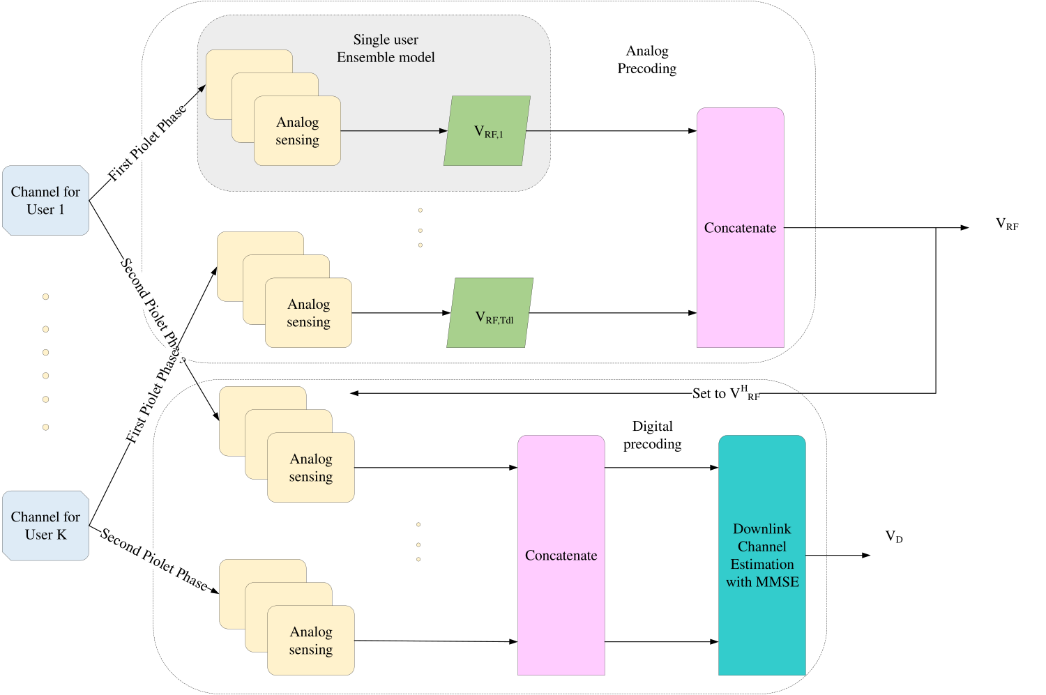
Figure 1: block diagram of the proposed for Hybrid Precoding for MIMO Systems
In the second part of the paper, we shift our focus to frequency-selective propagation scenarios, such as those encountered in OFDM systems. Here, a significant challenge arises as the analog precoder is common to all subcarriers, while digital precoders vary across subcarriers. To tackle this issue, we extend the separation of analog and digital precoder design. The analog precoder is determined using the ensemble deep learning approach, employing received pilots from all subcarriers, while digital precoders for each subcarrier are designed based on the corresponding estimated equivalent channel. To maximize the sum-rate expression, employed a hybrid optimization algorithm called CS-WaOA. This approach bridges the gap between deep learning and hybrid precoding, promising enhanced performance for Massive MIMO systems across various propagation scenarios.
System Model
Consider a TDD massive MIMO networks functioning in a frequency-selective mmWave environment, where a BS with antennas and RF chains uses OFDM broadcasting across subcarriers for serving single-antenna users. Downlink precoding is separated between the analogue and digital domains since the BS has a finite number of RF chains. Let be the precise symbol for user across subcarrier . The BS precodes the symbol vector using a per-subcarrier digital precoder , in order to deliver a downlink data stream of symbols . After that, it executes an inverted fast Fourier transform (IFFT) operation and adds a cyclic prefix of length LCP > , where is the maximum delay dispersion of the channel. Finally, the BS uses a wideband analogue precoding matrix called . Notably, we are unable to construct the analogue matrix on a per-subcarrier basis as the analogue step occurs after the IFFT module. The components of must also adhere to a constant modulus restriction, i.e., , where is the imaginary unit, because the analogue precoding stage is commonly performed using a network of phase shifters. Each user performs an FFT operation after receiving the signal, which includes cyclic prefix removal. The corresponding model is given by in mathematics:
(1)
Where is the downlink Gaussian noise, and are the received signal and frequency-domain channel of user at subcarrier , and is the column of . We impose a power constraint on the transmitted signal by taking and , where is the per-subcarrier power budget in the downlink. Aggregating the rates across the various subcarriers yields the overall achievable downlink rate for user k for this particular system. To put it another way, the sum of the rates across the different subcarriers yields the total achievable downlink rate for user .
(2)
In this study, the primary goal is to maximise the sum rate by designing the hybrid precoding matrices. The BS will need to gather channel-specific data to do this. In this study, we assume that the BS is unaware of the channels beforehand, but it is capable of acquiring noisy measurements of the channels during a pilot phase. Assuming that channel reciprocity is maintained and that a TDD operation can acquire the downlink CSI in the uplink direction, several assumptions are made. That use an uplink pilot transmission method that spans L time frames with each time frame containing OFDM symbols. Users broadcast orthogonal pilots, each of which is a unitary matrix, over the OFDM symbols in a single time frame, as determined by the rows of the matrices . This prototype program’s representation for the user. The BS detects pilot gearbox in the time frame using an analogue sensing matrix , where the matrix components fulfil . This is followed by a right-multiplication by of the signal that was received at the subcarrier. Because the pilots are orthogonal (i.e., ), the resultant received vector for the user in the time frame is given by:
(3)
Where PU is the users’ power budget per subcarrier in a particular time frame and is the comparable uplink noise. The total channel matrix for user throughout the frequency range is defined as .
(4)
As the total received matrices throughout the frequency range for user in time steps. The Eq. (3) is applied in Eq. (4) as,
(5)
Where is the overall sensing matrix and is a noise matrix whose columns are distributed as with , . The hybrid precoding design challenge for the system presented may be phrased as follows. Then build the analogue and digital precoding matrices in accordance with the noisy measurements received by the sensing matrix WRF at the BS.
(6)
Where is a function that converts the received pilots into the hybrid precoding matrices, with the goal of maximising the sum-rate expression. The following optimisation issue may be used to mathematically represent this:
Subject to
,
(7)
Due to its crucial function of condensing details about the user channels, the overall sensing matrix is included in the aforementioned issue as an extra optimisation variable. As a result, classic precoding schemes employ a two-step procedure in which user channels are first estimated before downlink precoding matrices are created using the estimated channels to try and heuristically tackle this issue. To overcome the drawbacks of the traditional method, the objective function in Eq. (7) is solved using the hybrid metaheuristic model called Cuckoo search based Walrus optimization algorithm (CS-WaOA).
Channel Model
A frequency-selective channel is used to represent the mmWave environment. In specifically, the Nc-point discrete Fourier transform (DFT) of its impulse response is used to indicate the channel of the user at the subcarrier.
(8)
Where the second equality results from the assumption that the channel response has a maximum delay spread . The is the discrete-time impulse response of the channel for user at time index . Assume that the sum of dominating pathways represents the discrete-time channel response, which follows a sparse model. After taking pulse shaping’s effects into consideration,
(9)
Where stands for the sampling period, for the normalised raised cosine pulse-shaping filter (i.e., = 1), and is assumed to be constant between users for simplicity. In addition, the complex path gain is represented by , the path delay is represented by , the uniformly distributed Angles of Departure (AoDs) in the elevation and azimuth are represented by and , and the array response vector is represented by . Each user receives a unique set of these channel settings that are produced individually. Additionally, we assume that the BS has a two-dimensional uniform planar array (UPA) with and antennas pointing in both the horizontal and vertical directions, where . Additionally, the antenna distances in both directions are , where . This configuration’s array response vector is as follows:
(10)
Where the array response vectors for a homogeneous linear array in both vertical and horizontal directions are , respectively.
(11)
(12)
Where is the wavelength.
Proposed Precoding Design
Splitting the entire L frame pilot phase into two independent phases of lengths and , where , in order to isolate the design of and . We use a ensemble model to transfer the pilots obtained during the initial pilot phase into the analogue precoding matrix in order to create the analogue precoder. Then fix the analogue beamformers and start the second pilot gearbox phase. Following that, the pilots from the second phase are utilised to estimate the low-dimensional equivalent channel and construct the digital precoding matrix using a traditional method without the need for further training. An ensemble model, which is the combination of MCRNN and LSTM are used for precoding.
MCRNN
This section discusses the structure of the proposed model as well as the specifics of its underlying assumptions. The input layer, convolutional layer, max pooling, and recurrent layer—also known as the output layer—have all been used as the foundation for the proposed model. The fully connected layer in this CNN architecture has been replaced with RNN, hence the suggested model has combined the convolutional and recurrent layers for the purpose of identifying zero-day threats. The following sections cover every one of these levels in more detail:
The CNN uses convolution layers and pooling layers to carry out layer-wise feature extraction in the design of the RNN for Zero Day attack detection. Because CNN does not require pre-processing or reconstruction of the original data, it overcomes the drawbacks of conventional machine learning techniques that require manually extracting data attributes. The weight-sharing aspects of the model also significantly reduce its complexity.
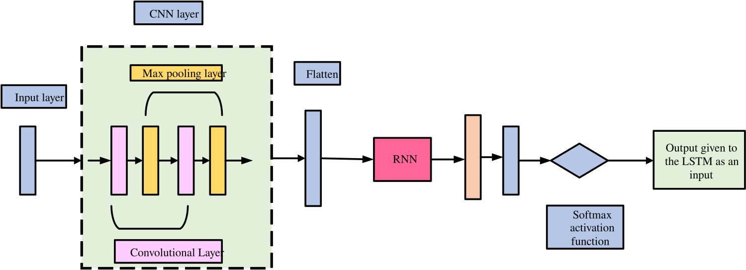
Figure 2: Hybrid CNN with RNN architecture
Figure 2 shows the construction of the CNN. The input data, which must be in two-dimensional form, is transformed by the kernel function. A series of convolution layers and pooling layers make up the hidden layer, where each layer’s input becomes its subsequent layer’s output. The input data may be used with this structure without many constraints, and the hierarchical expression of the input data can be correctly retrieved.
Convolutional Layer
The input data’s local properties are extracted using the convolution layer, which consists of a number of feature matrices. The number of free parameters may be greatly reduced since each feature matrix can be processed in parallel because it can be seen as a plane. Furthermore, the retrieved characteristics may be fully displayed because the convolution kernels differ depending on the plane. Following the convolution technique, the size of the output feature map is determined by the following Eq. (13) and Eq. (14):
(13)
(14)
Where the input image’s height is represented as , the resulting feature map’s height is , is the representation of input image’s width, the convolution operation’s padding is represented as , is the feature map’s width at the output side, the size of the filter is denoted as , and the convolution’ stride is denoted as .
Max Pooling
Max pooling (MP), a common pooling method, acts on the feature map side and selects the greatest value from a tiny patch of the input feature map. The specified values are then combined using MP to produce the output feature map. The resultant feature map size following the pooling technique may be calculated using the following Eq. (15) and Eq. (16):
(15)
(16)
Where is the size of the pooling area, the output feature map’s width is indicated by the prefix , the output feature map’s height is indicated by the symbol , the height of the input feature map’s is indicated by the symbol , the width of the input feature map’s is indicated by the letter w, and the width of the input feature map is denoted as .
RNN
By taking the place of the fully connected layer in the CNN for prediction, the RNN layer joins it. The reason for using the RNN layer to choose temporal features and the CNN to handle spatial features. Phrase parsing may be challenging and time-consuming, which is a disadvantage of the RNN. It’s intriguing to think that the same text may have many parse trees. For recursive neural networks, labelling the training data requires more time and effort than developing recurrent neural networks. It takes longer and more work to manually divide a statement into smaller portions than it does to label it.
The letter T represents trees, while the samples in the number N represent a tree’s leaves. Concatenated data including the potential child nodes of a tree are sent to the neural network. The neural network combines the two characteristics that were learnt through a nonlinear mapping to create a combined score and a parent feature. In mathematics, a parent is generated by concatenating the properties of the children in Eq. (17), that is, by using a nonlinear projection.
(17)
Where are the result of concatenating the child features x and y, is the neural network’s weight matrix, is its bias parameter, is a function that may be continually changed, and is the last parent attribute. Since its derivative can be expressed in terms of the main equation, the logistic sigmoid was chosen as the sign for this study. In order to decide if samples are fit for merging on the tree and, when necessary, whether they should be neighbours, the neural network learns a merging score. Just the samples with the highest score may be combined to create a binary tree. Eq. (18) is used to determine the score for the parent feature.
(18)
While the tree’s score can be increased K, it is possible to determine the parameters W, , and of the neural network,
arg (19)
Where θ is the representation of neural network parameter to calculate a score , and T are any potential trees produced by the aforementioned merging procedure. The outputs of the MCRNN model is given to the LSTM.
LSTM
The LSTM is a type of RNN that has memory blocks. Figure 5 depicts an illustration of a typical LSTM architecture. A forget gate (), an output gate (), and an input gate () make up its four gates. Cell () is also present. The long-term relationships between time steps in a data stream may be discovered using a stack of LSTM units. This kind of LSTM layer has two states: the hidden state, which keeps the output at time step , and the cell state, which retains the knowledge gained from prior time steps. The concealed and cell states are changed at each time step using the gates that have already been mentioned:
(20)
(21)
(22)
(23)
(24)
(25)
where the bias is denoted by the letter b, the weights matrix is denoted by W, the recurrent weights matrix is denoted by R, and the sigmoid activation function is denoted by σ. The structure of the LSTM model is shown in figure 3.
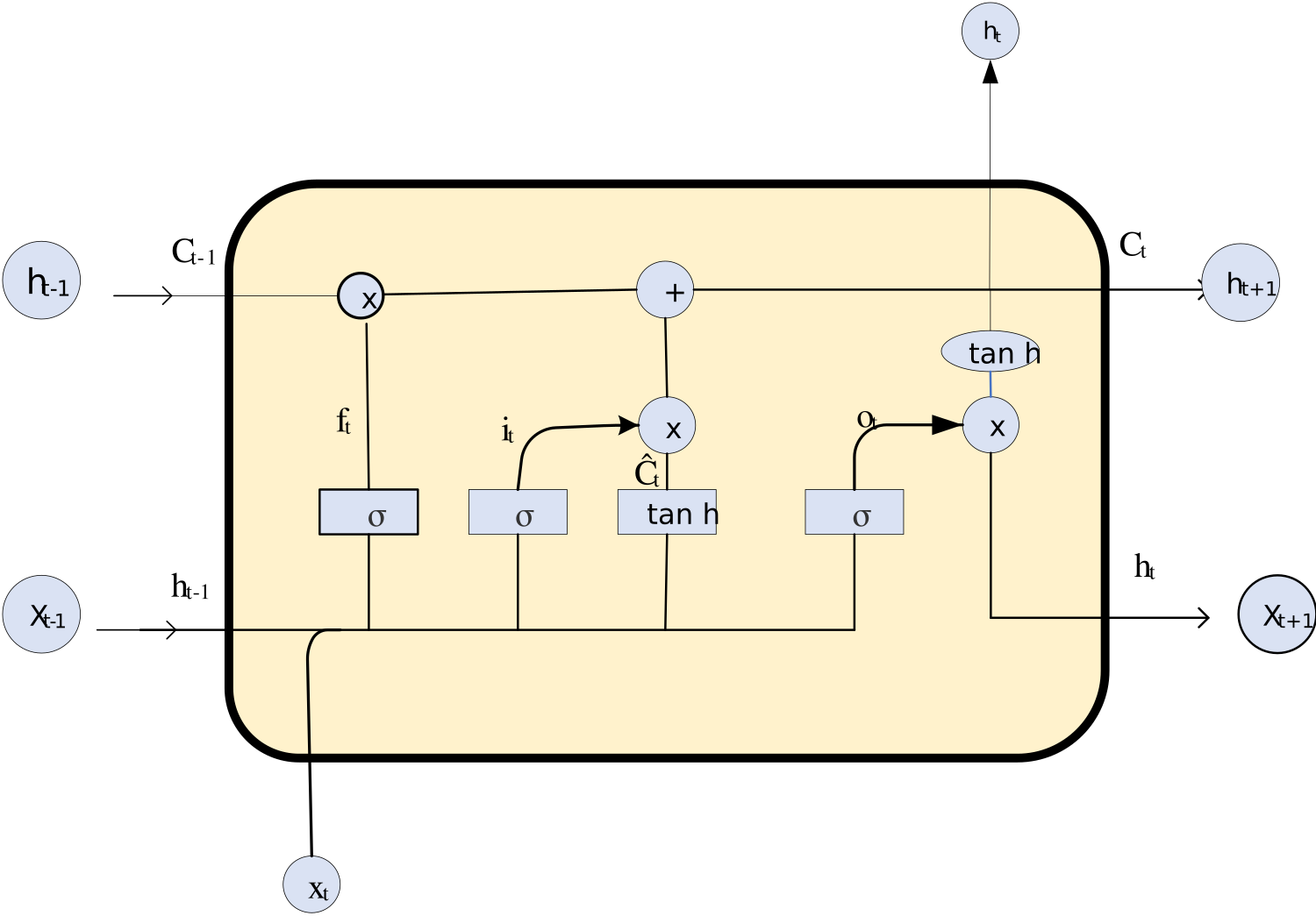
Figure 3: LSTM architecture with its basic units
The result is the weighted average of the CNN and LSTM results. A hybrid deep learning approach will be used to process the diagnostic report before being processed and sent to the anxious patient along with the doctor’s recommendations for a better prescription.
Precoding design at BS and downlink channel estimation
In contrast to FDD systems, time-division duplex (TDD) systems allow for the instantaneous acquisition of downlink channels through the reciprocity between uplink and downlink. By taking use of the AoA-delay reciprocity and the sparsity of mmWave massive MIMO channels, where the beam squint effect is carefully taken into account, we here present a unique downlink channel estimate technique for FDD systems with very minimal training overhead and limited user input.
In many scenarios, one may simply utilise a single RF chain to create a beam pointing in the desired direction for each multipath component without taking beam squint into account. A single RF chain cannot produce a beam given that the analogue precoders, or the phase setup in phase shifters, are typically fixed and constant throughout an OFDM block. Instead, a beam should be produced by frequency-dependent beamsteering vectors over various subcarriers. Signals in particular frequencies won’t be received by the designated users if beam squint is ignored. We suggest using multiple RF chains to collectively create the frequency-dependent beamforming vector across various subcarriers in order to solve this problem. The downlink channel model and user grouping are introduced in this part, and then we examine downlink channel estimates and our analogue and digital precoder architecture at the BS to handle the beam squint issue.
User grouping and the Downlink Channel Model
The downlink carrier wavelength and frequency are denoted as , respectively. One may directly formulate the downlink channel as,
(26)
Where may be calculated immediately using the uplink version that was obtained during the first parameter extraction process as,
(27)
Users should only be grouped in terms of AoAs since they are oblivious of route delays and are not required to synchronise with one another. In light of this, the separation between two downlink channels is described as,
(28)
In a similar manner, establish the equivalent guard distance , so that users and are allocated to the same downlink group if is greater than . A single OFDM block may not be able to entirely cover all users in a given spatial direction due to the constrained chains in transceivers with mixed digital/analog design. For the estimate of the downlink channel, use consecutive OFDM blocks. Multiple users in the same group will therefore get training at the same subcarriers within the OFDM block.
Use the notation to represent the total number of downlink groups and to represent the collection of user indices that make up group . Put in quotation marks to indicate user ‘s downlink channel at subcarrier . The received signal from antennas at the BS in the block from the user at the subcarrier in the group may be represented as
(29)
Where . The matching additive Gaussian noise is represented by the letters , and is the pilot symbol for the group, at the subcarrier, and in the block. Adding up the received signal for each subcarrier across blocks results in,
(30)
Where (31)
(32)
(33)
Beam Squint-Based Analogue and Digital Precoder Design
To create the analogue precoder, we first create a collection of all necessary steering vectors.
(34)
(35)
Following that, we use the following mutually orthogonal steering vector.
(36)
Where stands for the smallest integer that is not smaller than and stands for the largest integer that is not greater than . Assume that is an integer to preserve generality. Since , it is suggested that the downlink training process be finished in blocks. To roughly create every steering vector in , we anticipate to utilise the linear combination of the steering vectors in . In order to do this, the analogue precoder is created by stacking all of the steering vectors in into a matrix, with each column representing a single element (steering vector) in . is a diagonal matrix that serves as the digital precoder for the subcarrier.
(37)
Where is the spatial beamforming matrix at the user’s subcarrier to remove inter-user distortion between users in the similar cluster with
(38)
Where originates from the mutually orthogonal rows of the matrix with . This addresses the beam squint effect by employing various subcarriers and frequency-dependent beamforming vectors.
Downlink Channel Estimation with MMSE estimator
Consider the pilot symbols in pilot subcarriers to be all 1s and write . The LS estimate of downlink complex gains may be calculated as a result of the asymptotical symmetry among various user channels within the same group.
(39)
By substituting , can similarly create the downlink channel covariance matrix from Eq. (40). The can alternatively be determined by averaging earlier estimates of gains or even by substituting a single estimate of complex gains from the first uplink parameter extraction phase. The downlink complex gains’ MMSE estimate may be easily computed by defining for notational simplicity.
(40)
Where
(41)
Finally, the reconstruction and updating of user k’s downlink channel on all Nc subcarriers may be done as
Where (42)
The following summary of the suggested downlink channel estimate method is given as,
• Step 1: Extraction of the first uplink parameters: Pilots for orthogonal training are sent to the BS by users. The BS then employs the suggested technique derive the physical properties of each channel route.
• Step 2: Updates and comments are received using the downlink channel: Users are grouped by the BS and may be effectively trained in the same time-frequency band, where the BS broadcasts the downlink pilots. Users calculate downlink channel gains using the LS or MMSE estimators, and then they send those results back to the BS.
• Step 3: Reconstructed downlink channels: From the route delays and AoAs collected in Step 1 and the revised downlink channel gains in Step 2, the BS reconstructs the downlink channels.
Pilot Allocation
A logical trade-off exists between the number of pilots allotted to the analogue precoding design and those allotted to the digital precoding design. For a fixed , in instance, assigning more pilots to the analogue precoding design assures a strong analogue precoder but may harm the design of the digital precoder, and vice versa. According to the numerical simulations, the system gains more from using a higher (i.e., at the expense of a lower ). This is due to the fact that the analogue precoding step has more degrees of freedom than the digital precoding stage does. Spending more money on creating the analogue precoder is therefore more advantageous. In the simulations, we start with = and = 1 and look for the best option of .
Hybrid precoding for OFDM systems with frequency selection
Now let’s focus on the more widely applicable large MIMO system based on OFDM. With the following factors in mind, the suggested method should be expanded to the multicarrier case: (i) For all channels across Nc subcarriers, a single analogue precoder should be created; (ii) digital precoding should be done per-subcarrier. As before, we split the total precoding design into two parts: an analogue precoding design, where the analogue precoder is established using a direct mapping from the baseband signal received in the initial pilot transmissions, and a digital precoding design, which entails estimating the low-dimensional equivalent channel followed by linear precoding design. The ensemble model is trained to acquire a mapping from the baseband obtained pilots matrix across the entire frequency band (i.e., for the user) into the related analogue precoding vector. This will ensure that a common analogue beamformer is properly designed for the channels over the entire band. Additionally, because linear precoding is used to identify the appropriate digital precoder for each subcarrier because digital precoding occurs on a per-subcarrier basis, it is necessary to estimate the low-dimensional channel for each subcarrier. An intermediate stage, a normalisation layer, and a sensing stage comprise the network design in the OFDM case, which is comparable to the ensemble model for the single-carrier case. The primary distinction is that the ensemble model in the case of OFDM is intended to map the received data over all frequencies into a single analogue precoder. We suggest an intermediate step that consists of a convolutional layer followed by an FC stage to achieve this. In order to decrease the input dimension and take advantage of the channel’s correlation across the subcarriers, we use a convolutional layer, which also lowers the computing difficulty of the FC stage that follows. The columns of the received pilot matrix are specifically subjected to the application of convolutional filters, where each convolutional filter is a 1-D horizontal stripe of length and trainable parameters. The activation of a ReLU occurs after each filter output. In the end, feature vectors, each of length , are produced as the convolution result. After that, using the following FC step, the feature vectors are mapped into the unnormalized precoding vector.
Where the sensing stage and normalisation layer are equivalent to their single-carrier system’s DNN equivalents. Lastly, we employ the subsequent loss function:
(43)
Which generalizes the loss function Eq. (52).
Sum-rate maximization using CS-WaOA
Sum-rate maximization using CS-WaOA (Cuckoo Search with Walrus Optimization Algorithm) is a promising approach to enhance the performance of wireless communication systems, particularly in scenarios involving multiple users or antennas. The objective is to maximize the sum-rate, which represents the total data transmission rate or capacity of the communication system. CS-WaOA is designed to jointly optimize the precoding strategy and resource allocation to achieve this goal.
A population-based metaheuristic algorithm called CS-WaOA employs walruses as its searcher members. Each walrus in CS-WaOA stands for a potential solution to the optimisation issue. Therefore, the potential values for the issue variables depend on where each walrus is located in the search space. As a result, each walrus is a vector, and the walrus population may be mathematically represented using a structure known as the population matrix. During the earliest stages of CS-WaOA deployment, walrus populations are randomly initialised. Using Eq. (44), this CS-WaOA population matrix is generated.
(44)
Where represents the population of walruses, represents the walrus (candidate solution), represents the value of the choice variable recommended by the walrus, represents the total number of walruses, and represents the total number of decision variables. As was previously stated, each walrus is a potential solution to the issue, and the objective function of the issue may be assessed using the recommended values for each walrus’s contribution to the choice variables. The goal function’s estimated values, as determined by walruses, are given in Eq. (45).
(45)
Where is the result of evaluating the objective function’s value using the walrus and is the objective function vector. The best indicator of a prospective solution’s quality is its objective function values. The candidate solution considered to be the best member is the one that yields the best value for the goal function. As opposed to this, the worst member is the candidate solution that gives the objective function’s worst value. The best and worst members are changed in accordance with the revision of the objective function values made in each cycle.
Mathematical modelling of CS-WaOA
Based on the walrus’ normal behaviours, the process of updating its location in the CS-WaOA is divided into three stages.
Phase 1: Feeding strategy (exploration)
Walruses consume more than sixty different types of marine animals, including sea cucumbers, tunicates, soft corals, tube worms, prawns and numerous mollusks46. However, walrus favours benthic bivalve mollusks, especially clams, and forages by grazing on the ocean bottom while looking for and spotting prey with the help of its active flipper movements and sensitive vibrissae47. The largest, strongest walrus in the group leads the others in their quest for food. The quality of the objective function values of the candidate solutions is comparable to the length of the walruses’ tusks. As a result, the strongest walrus in the group is the best candidate solution with the best value for the goal function. The CS-WaOA’s exploration capacity in the global search is enhanced by the walruses’ search behaviour, which causes them to scan various parts of the search space. Under the direction of the most important member of the group, Eq. (46) and Eq. (47), the process of updating the position of walruses is mathematically modelled based on the feeding mechanism. This procedure starts by creating a new position for the walrus in accordance with Eq. (46). If this new location increases the value of the goal function, it replaces the prior position; this idea is modelled in Eq. (47).
(46)
(47)
Where denotes the newly generated position for the walrus based on the first phase, denotes its dimension, denotes the value of the walrus’ objective function, denotes random numbers from the range [0, 1], denotes the strongest walrus with the best value of the objective function, and denotes integers randomly chosen between 1 and 2.
Phase 2: Migration
Due to the warming of the air in the late summer, one of the normal behaviours of walruses is their movement to outcrops or rocky beaches. The CS-WaOA employs this migratory mechanism to direct the walruses in the search space to find appropriate regions in the search space. Using Eq. (48) and (49), this behavioural process is quantitatively modelled. This modelling makes the assumption that each walrus migrates to a different walrus location (chosen at random) in a different region of the search space. As a result, the suggested new position is first derived using Eq. (48). Then in accordance with Eq. (49), the new position will take the place of the walrus in the past if it increases the value of the goal function.
(48)
(49)
Where represents the newly generated position for the walrus based on the second phase, represents its dimension, represents its objective function value, and , } and represents the location of the chosen walrus to migrate the walrus towards it, representing its dimension, and representing its objective function value.
Phase 3: Escaping and fighting against predators (exploitation)
Polar bear and killer whale assaults are constant threats to walruses. The walruses move about in the area around where they are located as a result of their technique of evading and combating these predators. The CS-WaOA’s ability to utilise this aspect of walrus behaviour in the small search area surrounding potential solutions is enhanced. For the purpose of simulating this occurrence in CS-WaOA, a neighbourhood is assumed to be present surrounding each individual walrus, which is then given a random new position inside that neighbourhood using steps Eq. (50) and Eq. (51). Then, in accordance with Eq. (46), this new location replaces the prior position if the value of the goal function is increased.
(50)
(51)
(52)
Where is the newly generated position for the walrus according to the third phase, is its dimension, is its objective function value, is the iteration contour, and are the lower and upper bounds of the variable, respectively, and and are local lower and local upper bounds allowable for the dimension.
The first CS-WaOA iteration is finished, new values are computed for the location of the walruses, and the objective functions, depending on the execution of the first, second, and third phases. Up to the final iteration, updates and improvements to candidate solutions are made depending on the CS-WaOA processes as described in Eq. (46) to Eq. (52). The best candidate solution discovered during algorithm execution is presented by CS-WaOA as the solution to solve the stated objective function when the algorithm has finished running.
Results and Discussion
Evaluating the efficiency of a proposed model in comparison to existing techniques is a crucial step in assessing its performance. In the context of communication systems or signal processing, various metrics are commonly used to evaluate the performance of a model. The metrics mentioned, Bit Error Rate (BER), Mean Square Error (MSE), and throughput, are important for different aspects of model evaluation.
Comparison between existing deep learning techniques
In this section, a comprehensive evaluation of the performance metrics for the proposed method is conducted, and these results are rigorously compared with existing techniques, including CNN, RNN, LSTM, and Deep Neural Network (DNN). This evaluation process is essential to assess the effectiveness and superiority of the novel approach in solving the specific problem in channel sensing.
BER
The “Proposed” approach is continuously found to perform well in a thorough examination of various pilot sequence durations and signal-to-noise ratio (SNR) levels. For a pilot sequence length of 32, it constantly decreases in values from 1.618 at -10 dB SNR to 0.233 at 10 dB SNR, proving its durability under challenging circumstances. Although “CNN” and “RNN” provide competitive performance, they are not able to outperform the “Proposed” method in the majority of cases. The “LSTM” approach performs somewhat inconsistently, with its best outcomes coming from an SNR of 0 dB (0.529). However, “DNN” typically performs poorly, with the maximum value being 2.888 at -10 dB SNR.
When examining the effects of different pilot sequence durations, “Proposed” consistently performs better than the others. It continues to perform better than previous approaches for lengths of 64, with values ranging from 1.331 at -10 dB SNR to 0.028 at 10 dB SNR. With numbers ranging from 1.504 to 0.142, “DNN” regularly lags behind, demonstrating its dependability but relative performance deficit. While “CNN” and “RNN” perform competitively, with “CNN” occasionally displaying slightly lower values at certain SNR levels, “LSTM” exhibits some gains, especially at higher SNR levels.
When the length of the pilot sequence is increased to 128 and 256, “Proposed” continues to perform better. With values ranging from 1.285 at -10 dB SNR to 0.009 at 10 dB SNR for a length of 128, it consistently provides outstanding performance. While “CNN” and “RNN” exhibit competitive performance but still fall short of “Proposed,” “DNN” maintains its competitiveness but does not regularly outperform it. Although “LSTM” exhibits gain over the shorter pilot sequences, it still cannot compete with Proposed. The comparison of BER for various PL values are shown in figure 4.
|
|
PL=32 | PL=64 |
|
|
PL=128 | PL=256 |
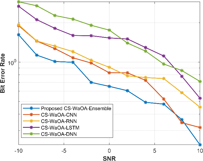
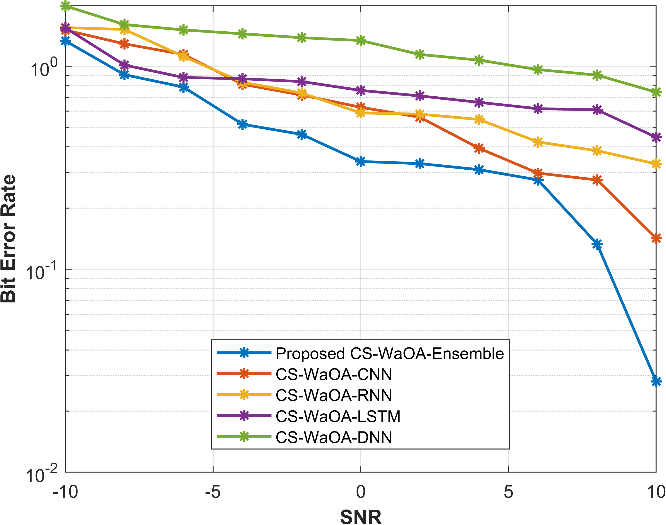
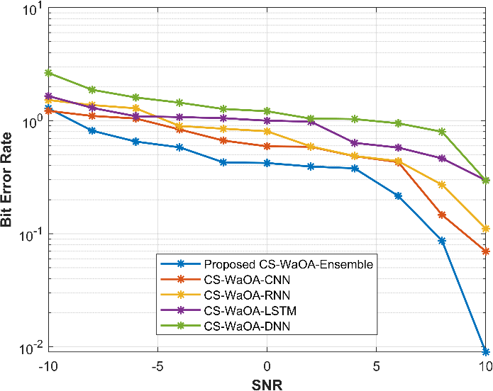
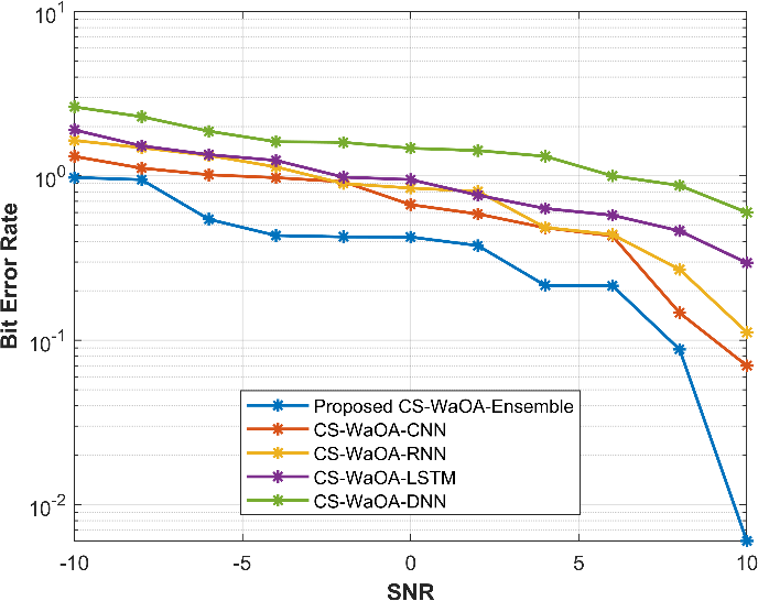
Figure 4: Comparison of BER values by changing the values of PL
The “Proposed” strategy consistently performs at the highest level throughout a range of SNR values and pilot sequence durations, with lower values suggesting higher levels of efficiency. As for competitors, “DNN” is the closest but often performs worse, while “CNN,” “RNN,” and “LSTM” provide competitive but inconsistent performance. The ideal approach ultimately depends on the demands and performance standards of the particular application, with “Proposed” being a solid and dependable option in many situations.
MSE
Different approaches perform differently for different durations of pilot sequences, depending on the signal-to-noise ratio (SNR) level, and varied patterns emerge. With values dropping from 1.333 at -10 dB SNR to 0.152 at 10 dB SNR, the “Proposed” approach consistently wins the competition for pilot sequence lengths of 32. While “Proposed” performs better than “CNN” and “RNN,” “LSTM” displays noticeable variance and performs best at an SNR of 0 dB (0.529). With a value of 2.888 at -10 dB SNR, “DNN” is last. With values ranging from 3.544 at -10 dB SNR to 0.121 at 10 dB SNR, “Proposed” maintains its lead at a pilot sequence length of 64. With values ranging from 4.99 to 0.673, “DNN” consistently performs worst. “CNN” and “RNN” perform similarly, and “LSTM” shows benefits at greater SNR levels.
With values ranging from 2.924 at -10 dB SNR to 0.028 at 10 dB SNR for a pilot sequence length of 128, “Proposed” retains its exceptional performance. Even while “Proposed” is still superior, “CNN” and “RNN” are in tight competition, while “LSTM” outperforms shorter pilot sequences. For a pilot sequence length of 256, “Proposed” retains its lead with values ranging from 2.613 at 10 dB SNR to 0.206 at -10 dB SNR. In comparison to “Proposed,” “CNN” and “RNN” perform competitively but still trail behind, while “LSTM” outperforms shorter pilot sequences. “DNN” always lags behind, with values varying from 5.305 to 1.949. Figure 5 displays the MSE comparison for a range of PL values.
|
|
PL=32 | PL=64 |
|
|
PL=128 | PL=256 |
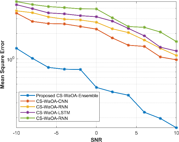
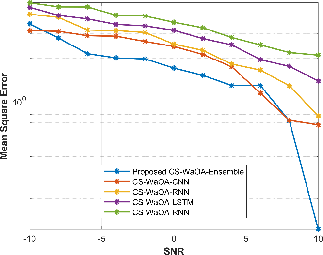
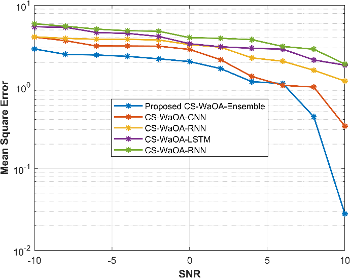
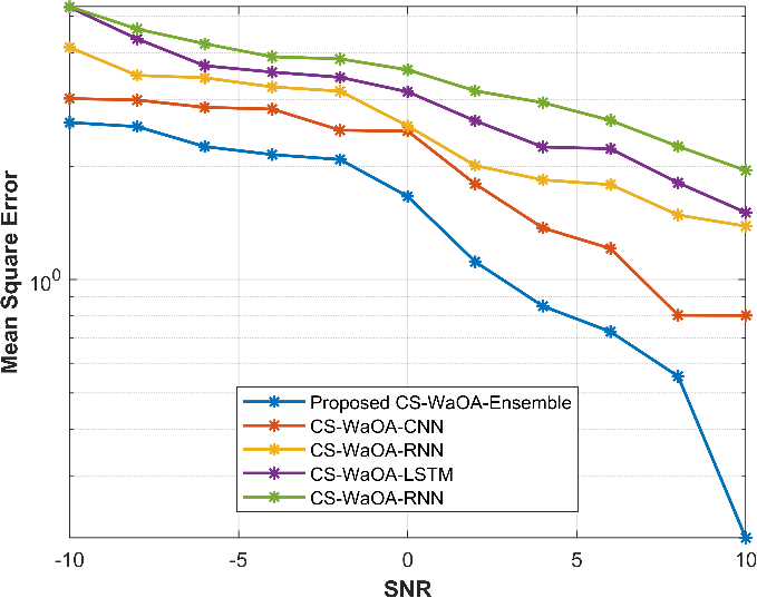
Figure 5: Comparison of MSE values by changing the values of PL
While “DNN” is its closest rival but regularly falls short, “Proposed” consistently exhibits the highest performance over a range of SNR levels and pilot sequence durations. The performance of “CNN,” “RNN,” and “LSTM” is competitive yet vary, and the optimum approach to use in each situation depends on the application-specific needs.
Throughput
When the performance is examined at various signal-to-noise ratio (SNR) levels for varied pilot sequence durations, a number of tendencies become apparent. With values ranging from 0 at 0 dB SNR to 24.005 at 8 dB SNR for a pilot sequence length of 32, the “Proposed” approach consistently performs well. While “CNN” and “RNN” perform similarly, they are not as well as “Proposed.” With the best outcome at 0 dB SNR (7.094), “LSTM” exhibits a noticeable range in performance. With the greatest value of 2.888 at -10 dB SNR, “DNN” trails behind. With values ranging from 0 at -10 dB SNR to 20.005 at 10 dB SNR, “Proposed” continues to dominate when the pilot sequence length is increased to 64. “DNN” lags behind continuously, showing a range of values from 20.005 to 0.673. “CNN” and “RNN” both perform favourably, with “LSTM” showing gains at greater SNR levels.
At a pilot sequence length of 128 and values ranging from 0 at -10 dB SNR to 19.001 at 10 dB SNR, “Proposed” continues to be the better performance. While “LSTM” displays improvements over shorter pilot sequences, “CNN” and “RNN” are closely matched but still fall short of “Proposed.” “Proposed” retains its supremacy for pilot sequence lengths of 256, with values ranging from 0 at 0 dB SNR to 19.003 at 8 dB SNR. While “LSTM” displays gains over shorter pilot sequences, “CNN” and “RNN” compete well but still fall short of “Proposed.” Values from 19.003 to 0.206 indicate that “DNN” routinely lags behind. Figure 6 displays the comparison of throughput for different PL levels.
|
|
PL=32 | PL=64 |
|
|
PL=128 | PL=256 |
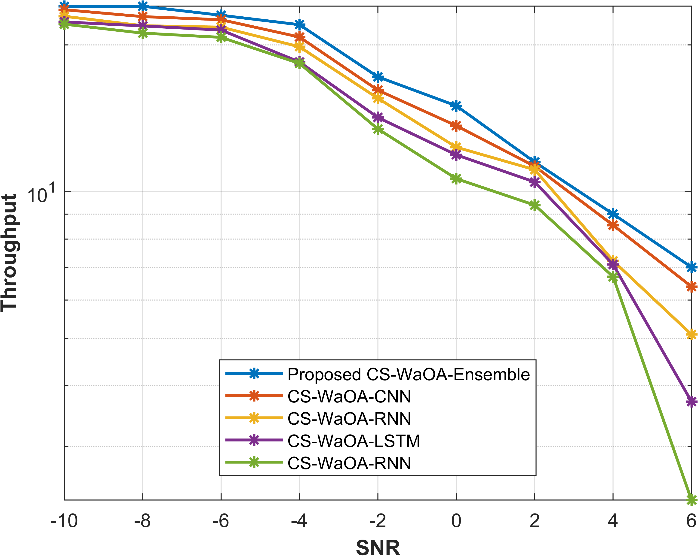
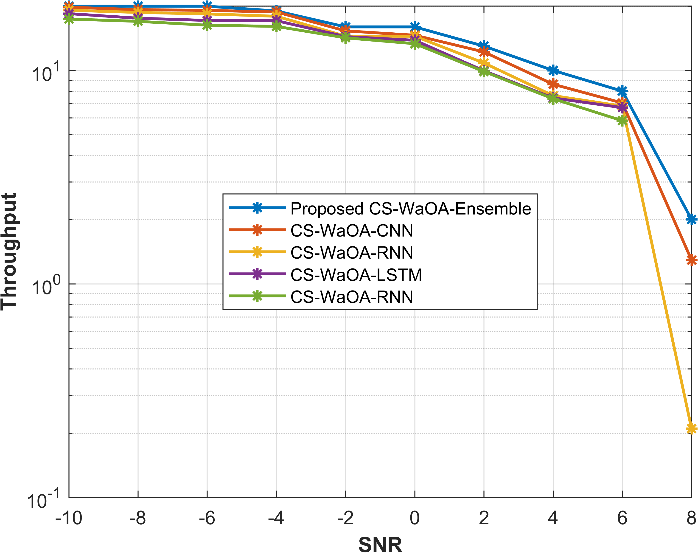
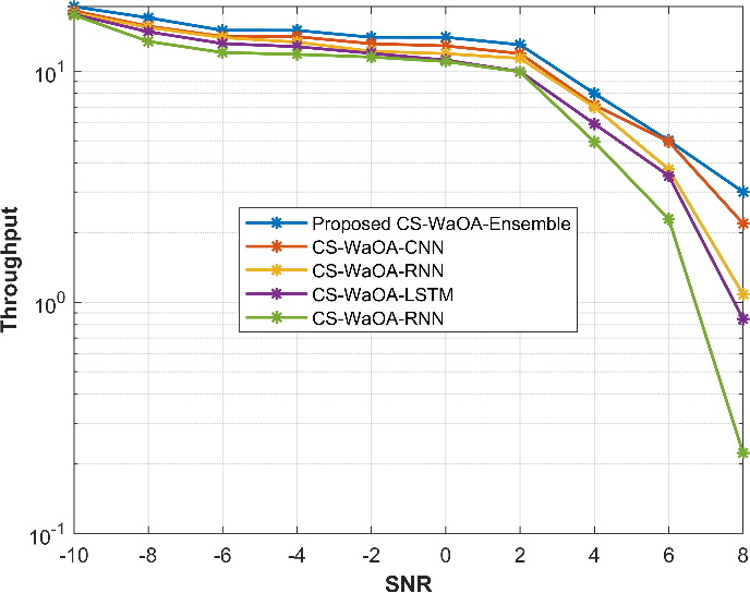
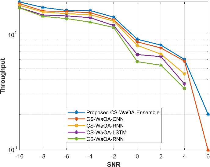
Figure 6: Comparison of throughput values by changing the values of PL
Comparison between existing optimization techniques
This section compares the suggested optimisation to current methods such as CSO, WaOA, Particle Swarm Optimisation (PSO), and Ant Colony Optimisation (ACO). By assuming that 64 is the Pilot sequence length value, the metrics of BER, MSE, and throughput are calculated. In figure, the graphs are displayed. Figure 7 presents a comparison of BER, MSE and throughput values for different values of PL=32 and the comparison is between various existing optimizations.
|
|
BER | MSE |
| |
Throughput | |
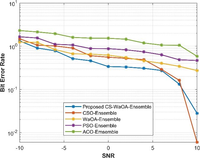
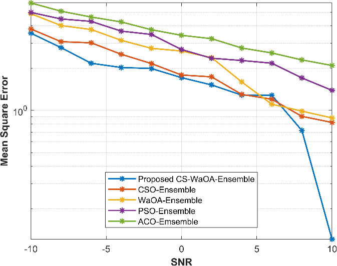
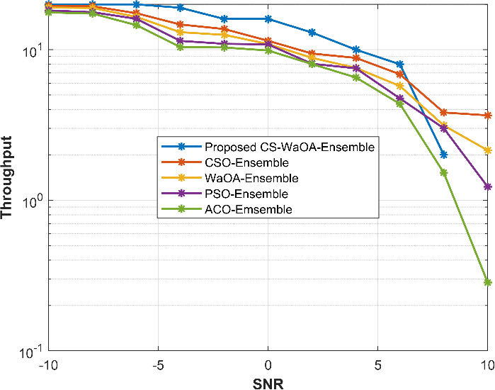
Figure 7: Comparison of BER, MSE and throughput values for different optimizations
A comparison of five distinct communication or signal processing algorithms, including “Proposed,” “CSO,” “WaOA,” “PSO,” and “ACO,” is shown in the picture. These algorithms operate within a range of Signal-to-Noise Ratios (SNR) from -10 to 10. Three important measures are used to assess their performance: throughput, mean squared error (MSE), and bit error rate (BER). Lower values of BER indicate higher performance since they assess the accuracy of digital data transfer. The “Proposed” technique has a BER of 1.331 at SNR -10, which indicates that around 1.331% of sent bits are received wrongly. The BER reduces with SNR as it reaches a relatively low value of 0.028 at SNR 10, suggesting extremely precise data transmission. The other algorithms in the diagram have comparable meanings.
Lower values of MSE imply greater performance when evaluating the quality of the signal or data reconstruction. The average squared difference between estimated and genuine signals for the “Proposed” method is 3.544 at SNR -10. Improved signal estimating or data reconstruction is indicated by a general reduction in the MSE with increasing SNR. The MSE values of the other methods are also used to assess them. Higher numbers indicate better throughput, which is a measurement of the rate of data transfer. For the “Proposed” method, a throughput of 0 at SNR -10 denotes that there was no data transfer because of the low SNR. However, when SNR grows, throughput also improves, reaching a maximum value of 20.005 at SNR 10, indicating extremely effective data transfer. The throughput metrics for the alternative methods follows a similar pattern.
Conclusion
This paper presents a novel approach to optimize Massive MIMO systems, effectively addressing the challenges of explicit channel estimation in various propagation scenarios. In the first part, we focused on frequency-flat mmWave propagation, where we introduced ensemble deep learning, including LSTM and MCRNN, to map received pilot signals to analog and digital precoders. This approach outperformed traditional methods that separate channel estimation and downlink precoding.
In the second part, we addressed frequency-selective propagation, extending the separation of analog and digital precoder designs. We applied hybrid optimization, combining Cuckoo search and Walrus optimization, to maximize the sum-rate expression. This approach bridges the gap between deep learning and hybrid precoding, promising significant performance improvements in Massive MIMO systems across diverse scenarios. This work offers a robust and adaptable solution for optimizing MIMO systems, potentially transforming wireless communication technology in real-world applications. Further research and implementation can harness its full potential.
References
Qi, X., Chen, Y., Jian, R. and Wang, J., 2022. Two-level-enforced security with hybrid precoding for multicast massive MIMO wiretap systems. Physical Communication, 54, p.101817.
Chataut, R. and Akl, R., 2020. Massive MIMO systems for 5G and beyond networks—overview, recent trends, challenges, and future research direction. Sensors, 20(10), p.2753.
Raja, R.A. and Vijayalakshmi, B., 2023. Improved spectral efficiency in massive MIMO ultra-dense networks through optimal pilot-based vector perturbation precoding. Optik, 273, p.170370.
Audu, W.M. and Oyerinde, O.O., 2022. Iteratively reweighted super-resolution channel estimation in hardware-impaired hybrid-precoded MM-wave massive MIMO systems using dual SVD and Marquardt’s global search. Digital Signal Processing, 120, p.103308.
Mishra, A., Mao, Y., Thomas, C.K., Sanguinetti, L. and Clerckx, B., 2022. Mitigating intra-cell pilot contamination in massive MIMO: A rate splitting approach. IEEE Transactions on Wireless Communications.
Papazafeiropoulos, A.K., Papageorgiou, G.K., Kolawole, O.Y., Kourtessis, P., Chatzinotas, S., Senior, J.M., Sellathurai, M. and Ratnarajah, T., 2021. Towards the assessment of realistic hybrid precoding in millimeter wave MIMO systems with hardware impairments. IET Communications, 15(12), pp.1606-1619.
Deshpande, S., Sharma, P., Aggarwal, M. and Ahuja, S., 2021. Mitigating pilot contamination in Rician faded massive MIMO 5G systems using enhanced zero forcing precoding and ring partitioning. Physical Communication, 49, p.101467.
Huang, H., Song, Y., Yang, J., Gui, G. and Adachi, F., 2019. Deep-learning-based millimeter-wave massive MIMO for hybrid precoding. IEEE Transactions on Vehicular Technology, 68(3), pp.3027-3032.
Al-Kamali, F. and D’amours, C., 2022. Low-complexity hybrid precoding for subarray architecture mmWave MIMO systems. IEEE Access, 10, pp.74921-74930.
Das, D., Bora, P.K. and Bhattacharjee, R., 2021. Automatic modulation classification over MIMO amplify and forward (AF)-relay fading channels. Physical Communication, 47, p.101399.
M. Elmagzoub, H., 2020. On the MMSE‐based multiuser millimeter wave MIMO hybrid precoding design. International Journal of Communication Systems, 33(11), p.e4409.
Zheng, Z., Zhang, J., Wu, X., Liu, D. and Tian, L., 2019. Zero-forcing precoding in the measured massive MIMO downlink: how many antennas are needed?. International Journal of Antennas and Propagation, 2019, pp.1-10.
Park, W. and Choi, J., 2022. Hybrid precoding and combining strategy for MMSE-based rate balancing in mmWave multiuser MIMO systems. IEEE Access, 10, pp.88043-88057.
Hong, S.E., 2021. On the effect of shadowing correlation and pilot assignment on hybrid precoding performance for cell-free mmWave massive MIMO UDN system. ICT Express, 7(1), pp.60-70.
Lavdas, S., Gkonis, P.K., Zinonos, Z., Trakadas, P., Sarakis, L. and Papadopoulos, K., 2022. A machine learning adaptive beamforming framework for 5G millimeter wave massive MIMO multicellular networks. IEEE Access, 10, pp.91597-91609.
Ding, T., Zhao, Y. and Zhang, L., 2021. Hybrid precoding for mmWave massive MU-MIMO systems with overlapped subarray: A modified GLRAM approach. ICT Express, 7(4), pp.460-467.
Al-Kamali, F., D’Amours, C. and Chan, F., 2022. Hybrid precoding for mmWave MIMO systems with overlapped subarray architecture. IEEE Access, 10, pp.130699-130707.
Subitha, D., Poonkuzhali, P., Chandra, I. and Hemanth, P.V., 2023. Hybrid precoding algorithm for massive MIMO system with imperfect channel knowledge. Materials Today: Proceedings, 80, pp.3235-3239.
Uwaechia, A.N. and Mahyuddin, N.M., 2021. A novel committee machine hybrid precoding and combining algorithm for mmWave massive MU-MIMO systems. Physical Communication, 46, p.101326.
Ullah, K., Alohali, M.A., ul Haque, M.I., Mahgoub, H., Nafie, F.M., Assiri, M., Nauman, A. and Chowdhry, B.S., 2023. Hybrid precoding design for secure smart-grid enabled MIMO wireless communications in Industry 5.0. Journal of King Saud University-Computer and Information Sciences, 35(7), p.101579.
Khalid, S., Mehmood, R., Abbas, W.B., Khalid, F. and Naeem, M., 2020. Joint transmit antenna selection and precoding for millimeter wave massive MIMO systems. Physical Communication, 42, p.101137.
Wang, S., He, M., Zhang, Y. and Ruby, R., 2021. Equivalent channel-based joint hybrid precoding/combining for large-scale MIMO systems. Physical Communication, 47, p.101287.
Bai, X., Liu, F., Du, R., Kan, X., Xu, Y. and Zhang, Y., 2019. ROD-based hybrid TH precoding and combining for mmWave large-scale MIMO systems. Digital Signal Processing, 93, pp.102-114.
Du, J., Wang, Z., Zhang, Y., Guan, Y. and Jin, L., 2021. Multi-user hybrid precoding for mmWave massive MIMO systems with sub-connected structure. EURASIP Journal on Wireless Communications and Networking, 2021(1), pp.1-21.
Cite This Work
To export a reference to this article please select a referencing stye below:

Academic Master Education Team is a group of academic editors and subject specialists responsible for producing structured, research-backed essays across multiple disciplines. Each article is developed following Academic Master’s Editorial Policy and supported by credible academic references. The team ensures clarity, citation accuracy, and adherence to ethical academic writing standards
Content reviewed under Academic Master Editorial Policy.