Crop Leaf Disease Detection Using VersaNet and Semantic Segmentation

Abstract

Crop leaf diseases can significantly affect agricultural productivity. Addressing this challenge, we present a comprehensive methodology for precise leaf disease detection. Our proposed approach combines advanced techniques in image processing, segmentation, feature extraction, and deep learning to achieve accurate and versatile identification of disease-affected regions. In the first step, we perform meticulous image pre-processing, encompassing data augmentation for diversity, normalization for consistent inputs, color enhancement for improved quality, and noise reduction for clarity. This sets the stage for robust analysis. For accurate region delineation, we employ Semantic Segmentation, leveraging the power of the U-Net architecture enriched with skip connections and dilated convolutions. This method effectively captures local and global context, ensuring precise separation of healthy and affected regions. Feature extraction encompasses various aspects. We tap into color features, utilizing Color Space Transformations such as RGB, HSV, and LAB, to identify distinct color patterns indicative of diseases. Symmetry and regularity metrics enable the detection of irregularities associated with disease presence. Texture features, extracted through advanced techniques like Improved LrTP, capture unique spatial arrangements resulting from diseases. The subsequent feature selection step is enhanced by a hybrid optimization approach integrating the Marine Predator Algorithm (MPA) and Mountain Gazelle Optimizer (MGO). This synergistic strategy pinpoints the most relevant features, refining the focus on discriminative characteristics. The pinnacle of our methodology is the introduction of the VersaNet deep learning framework. VersaNet harmonizes the power of LeNet, RNN, and EfficientNet. This fusion maximizes the model’s ability to comprehend various data modalities, ensuring robust performance across diverse scenarios. Our proposed methodology is implemented using Python, a versatile tool that aligns seamlessly with the entire workflow. Through extensive experimentation, we demonstrate the efficacy of our approach on real-world crop datasets. Versatile in its capabilities and accurate in its results, our methodology paves the way for proactive disease management in agriculture, ultimately contributing to enhanced crop yield and global food security.

Introduction

Computer vision & machine learning techniques are used to identify crop leaf diseases in crop plants. By analyzing images of leaves and using advanced algorithms, the system can accurately diagnose diseases early, enabling farmers to take timely and targeted actions to prevent extensive crop damage and increase overall agricultural productivity. Plant diseases can strike leaves during crop farming, causing significant production losses and financial impacts in the market [1]. Therefore, enhanced monitoring, detection, and prediction of crop diseases are critical to minimize agricultural losses and improve crop productivity [2]. The imaging technique measures the diseased area & applies adaptive operation to an appropriate color picture channel. Using grey level slicing, peach crop bacterial spot disease can be segmented and identified [3]. The Automatic Image Segmentation Algorithm (AISA), which is based on the GrabCut algorithm, is designed to eliminate background information from images while maintaining the disease spot [4]. Leaf diseases significantly affect crop yield and quality. Proper diagnosis and classification are crucial for early intervention and improved tomato production [5].

The restructured residual dense network, a novel model for identifying tomato leaf disease, merges deep network and dense residual, improving calculation accuracy and information flow [6] and an enhanced Faster RCNN for tomato leaf disease detection, utilizing a bounding box clustering using a depth residual network for k-means clustering and  feature extraction [7]. A novel deep CNN, based on EfficientNet, was fine-tuned for detecting unhealthy tomato and healthy and leaf images and the challenge of scaling plant disease detection due to sample selection bias is addressed with a Bayesian deep learning-based probabilistic programming technique and uncertainty quantification [8][9]. There are three deep learning meta-architectures: SSD, RFCN, and Faster RCNN were implemented with TensorFlow’s object detection framework to identify plant disease using controlled environment dataset [10].

Despite the advancements, Identification of the mildew disease in pearl millet using transfer learning as well as feature extraction may face challenges due to limited specific dataset availability and the need for efficient data analysis in precision agriculture, this approach seeks to enhance disease detection [11]. The primary challenge in automated plant disease identification using this strategy is inadequate representative image databases for diverse conditions. Data augmentation mitigates but doesn’t fully replicate practical diversity [12]. Although crop disease detection lacks comprehensive research, deep learning holds unexplored potential. Challenges include lengthy training times due to limited GPUs, solvable with high-speed GPUs [13] . Despite advancements, plant disease classification requires more robust models due to diverse conditions [14]. Hence, to grasp plant disease symptoms, presented an alternative approach, training models using disease names instead of crop-disease pairs [15].

The following is the main contribution of this research

To preprocess the image, the data is augmented by applying rotation, scaling, flipping and brightness adjustment, normalization, color enhancement, and noise reduction.

U-Net architecture with skip connection is used for semantic segmentation.

To extract the features, some meaningful features are derived like color symmetry& regularity & texture by improving LrTP.

To select the features hybrid optimization is carried out by combining Marine Predator Algorithm and Mountain Gazelle Optimization.

For model selection, a new deep learning framework has been referred to as VersaNet by combining LeNet, Modified RNN, and EfficientNet.

The research has been divided into five sections: an introduction; a complete literature review; a description of the suggested approach; an explanation of the findings and discussions; and a conclusion of the research’s findings in section five.

Literature Review

In 2020, Anami and Malvade et al. [16] have developed automated detection of abiotic and biotic stressors in rice crops using a deep convolutional neural network (DCNN) architecture using field images. The approach employs the classification using a pre-trained VGG-16 CNN model. However, potential drawbacks include limited adaptability to various growth stages and challenges in handling diverse stress patterns.

In 2020, Ai and Sun et al. [17] have aimed to enhance agricultural digitization, mitigate the impact of pests and diseases on crops, and boost overall crop yield. This involved leveraging technological advancements to effectively manage and counteract the damaging effects caused by pests and diseases, ultimately leading to improved agricultural productivity and output.

In 2020, Chen and Chen et al. [18] have explored transfer learning for deep CNNs to increase the capacity for learning about mild lesion symptoms. For recognizing photos of plant diseases, the INC-VGGN innovative deep learning architecture had been suggested. By adding a new convolutional layer that incorporates batch normalization and the Swish activation function, the pre-trained VGGNet was modified. For the purpose of reducing the dimension of the feature map, two Inception modules were substituted for fully connected layers, followed by a global pooling layer.

In 2021, Tiwari and Joshi et al. [19] have used an approach based on deep learning is used to identify and categorize plant diseases from various resolutions of leaf photos. The training of a dense convolutional neural network (CNN) architecture used a large dataset of plant leaves collected from different nations. The study encompassed six crops spanning 27 categories under both laboratory and on-field conditions, addressing complex and challenging intra-class and inter-class variations through the dense neural network.

In 2020, Sharma and Berwal et al. [20] have explored the practicability segmented as well as labelled images rather than whole images when training a convolutional neural network (CNN) model. The model’s performance on independent datan enhanced dramatically, going from 42.3% to 98.6%, when the same CNN model was trained with segmented images (S-CNN) as opposed to full images (F-CNN).

In 2019, Nagasubramanian and Jones et al. [21] have introduced Hyperspectral imaging emerged as a promising technique for plant disease identification. The abundant information within hyperspectral data cubes was harnessed using a pioneering 3D deep convolutional neural network for disease identification. The model was examined to generate interpretable insights. The study centered on charcoal rot, a significant soil-borne fungal disease impacting global soybean crop yields.

In 2020, Waheed and Goyal et al [22have suggested a deep-learning system to monitor crop health, resulting in better agricultural output in terms of both quantity and quality. In comparison to current CNN architectures like XceptionNet,EfficientNet, NASNet, and VGG19Net, the optimised DenseNet model obtained 98.06% accuracy with less parameters. The optimized model’s performance was evaluated using two quality metrics: time and accuracy.

In 2020, Jiang and Lu et al. [23] have introduced images of rice leaf disease have been processed using convolutional neural networks to extract features. The SVM approach were subsequently used for disease categorization and prediction. The 10-fold cross-validation method was used to determine the SVM model’s ideal parameters, improving the process’s accuracy and dependability for spotting diseases.

In 2020, Zhao and Liu et al. [24] have introduced an automated crop disease recognition system within agricultural IoT, leveraging the MultiContext Fusion Network to enhance crop disease identification. The approach involved Convolutional Neural Networks (CNNs) to incorporate contextual features as prior knowledge, enhancing recognition accuracy. MCFN integrated contextual information and high-level visual features, significantly improving crop disease identification performance.

In 2019, Arsenovic and Karanovic et al. [25] have introduced encompassing real-world leaf images captured from different angles and weather conditions, enhancing model accuracy and practicality. Augmentation techniques and GAN were employed to tackle the challenge of limited examples and overfitting. The PlantDiseaseNet, for the purpose of detecting plant diseases, a two-stage design was designed.2.1 Problem Statement

Table 1: Aim and Drawback of the previous research

Proposed Methodology

The proposed methodology presents a systematic approach to efficiently classify crop leaf diseases from images. Initial image pre-processing involves techniques like data augmentation, normalization, color enhancement, and noise reduction to ensure diverse and high-quality data. The segmentation phase accurately isolates disease-affected regions using advanced methods such as the U-Net architecture. Feature extraction encompasses color, symmetry, and texture attributes, highlighting disease cues. A hybrid optimization approach employing the Marine Predator Algorithm and Mountain Gazelle Optimizer selects pertinent features. The novel VersaNet framework combines LeNet, RNN, and EfficientNet for precise disease classification. This comprehensive approach ensures accurate crop disease identification through a streamlined process as depicted in Fig. 1.

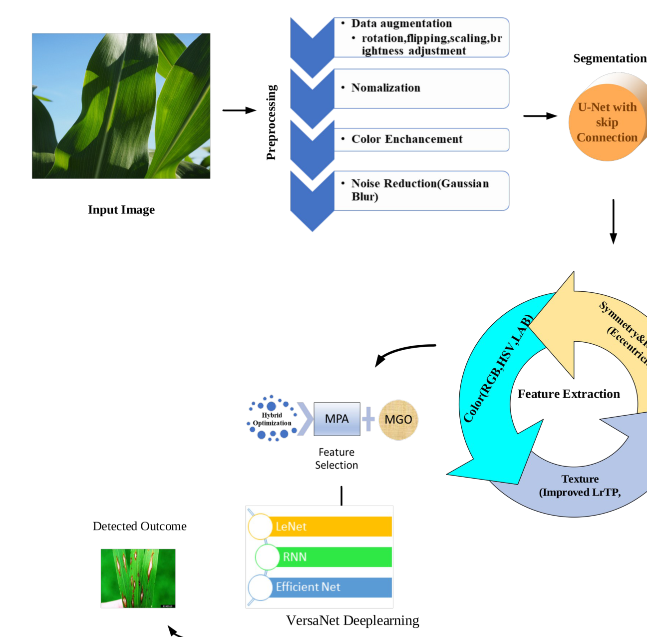
Figure 1: Overall flow diagram of the proposed model

Preprocessing

In this research, the initial phase of image pre-processing includes different methodologies. Rotations, scaling, flips, and brightness modifications are included in data augmentation procedures to add variation to the dataset and improve the model’s capacity for generalization. By matching the pixels within a predetermined spectrum via pixel value normalization, uniformity is created. Color enhancement techniques are used to combat color inconsistencies caused by various lighting and camera conditions, maintaining uniform data quality. Following noise reduction, which makes use of Gaussian blur and filters to improve image precision, increases the applicability of the images for the best training.

Data Augumentation

In Preprocessing, Data augmentation is a machine learning strategy that uses a number of significantly altered copies of the same existing data to train machine learning models, hence reducing overfitting when training a machine learning model. The term “image augmentation” refers to a variety of transformations, including random flipping, cropping, rotating, zooming, resizing, stretching, and affine changes.

Rotation

Random rotation is a common approach that repositions objects in the frame by applying arbitrary clockwise or anticlockwise rotations. Notably, in cases involving object detection, bounding boxes must be recalculated in order to appropriately represent the changing item.

Scaling

In Data augmentation, scaling is an enhancement approach in which the image’s short size within a dimension range is selected at random.

Flipping

In Data augmentation, Reversing pixels horizontally or vertically creates a mirror effect and this is referred to as mirroring or flipping. When an image is rotated horizontally, pixels with coordinates (x, y) become (width – x – 1, y) in the updated version. By adding mirrored perspectives, this strategy increases dataset variation and enhances model reliability.

Brightness Adjustment

Brightness adjustment is an important aspect of image preprocessing for data augmentation. It includes adjusting the intensity of pixel values throughout an image to control brightness. The overall illumination of the image is precisely controlled by uniform increments or decrements in pixel values. This technique raises dataset variation and strengthens the model’s adaptability to various illumination conditions.

Normalization

In preprocessing, Normalization is an approach used in image processing to alter the intensity range of pixels. Examples of applications would be glare-damaged pictures. Stretching the contrast or stretching the histogram are two names for normalization. Data preprocessing enhances machine learning algorithms’ efficiency and precision approach known as normalization, which transforms information in a dataset to a common scale.

x_norm=(x-x_min)/(x_max-x_min) (1)

Color Enchancement

In the preprocessing stage of an image, color enhancement is essential. By minimizing variances brought on by various lighting conditions and camera settings, it incorporates advanced processes that harmonize and improve color constancy. The quality of the data is improved by correcting color discrepancies by using specialized algorithms. By enhancing the dataset, this improvement makes it possible to classify and detect diseases in agricultural crop photos with greater accuracy.

Noise Reduction

Noise reduction stands as a frequent undertaking in digital image processing, focusing on the elimination of undesirable or stochastic pixel value fluctuations within an image. This procedure aims to refine image quality by mitigating irregularities, enhancing overall clarity, and aiding in improved visual interpretation and analysis. By removing noise with filters and Gaussian blur, researchers may improve image clarity and make it more suitable for training.

Gaussian Blur

Image blurring using a Gaussian function is referred to like a Gaussian blur. This is a typical effect in graphics software and is typically used to minimise visual noise and detail. The bokeh effect produced by an out-of-focus lens or the shadow of an item in normal illumination are markedly different from the smooth blur produced by this blurring technique, which gives the impression that you are seeing through a translucent screen.

gXY=(1)/(√(2π )σ)e^{-(X2+Y2)/(2σ2)} (2)

Eq.(2) X stands for the horizontal axis distance, Y for the vertical axis distance, and for the Gaussian distribution’s σ standard deviation.transparent screen, which stands out significantly from the bokeh effect produced by an out-of-focus lens or the shadow of an object under normal lighting.

Segmentation

In this research, semantic segmentation is used in the process to distinguish precisely between disease-affected and healthy regions. Cutting-edge approaches, such as the proposed U-Net design with skip connections and dilated convolutions ensure accurate separation.

U-Net

The U-Net architecture stands out for its ability to yield robust outcomes, particularly with scant data, exploiting feedback across layers from input to output. Comprising encoding and decoding segments, this choice is motivated by the study’s limited dataset. For enhanced model efficacy, structural rearrangements and an encoder-shift to decoder-decoder with skip connections, employing a pre-trained ResNet network, can be pursued. Such adaptations empower the model for superior performance and capitalize on transfer learning advantages.

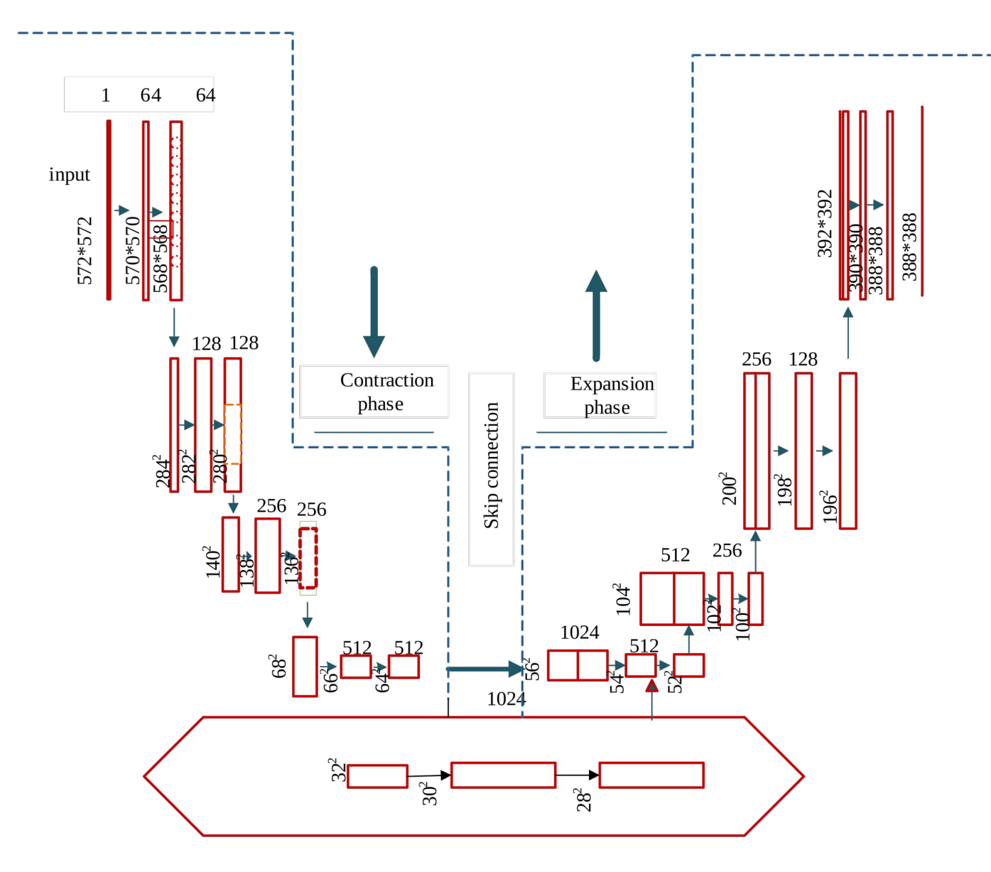
Figure 2: U-Net Architecture

Initial pooling reduces information in the core U-Net design, potentially eliminating important pixel window data and insights. To mitigate this, a higher-stride convolutional layer is used in place of the pooling layer, storing discarded data while preserving important information.

By omitting high-level input image information, the encoder segment of U-Net collects context. It downsamples spatial dimensions while enhancing feature channels and consists of many convolutional layers with pooling. By doing this, the image’s context and coarse-grained data are protected.

A segmentation map that is the same size as the original input can be up-sampled by U-Net’s decoder, on the other hand. It recovers spatial dimensions via transposed convolutions or interpolation from low-resolution feature maps obtained by the encoder. It links encoder and decoder feature maps using skip connections, maintaining fine features and local context, and improving segmentation quality.

Residual Block with Skip Connection

In the MDA-Unet architecture, the incorporation of Residual Blocks with skip connections plays a pivotal role in addressing the vanishing gradient issue and empowering the training of deeper neural networks. These blocks follow a structured sequence: initially, two 3×3 convolutional layers are applied, followed by ReLU activation and batch normalization . Crucially, a skip connection is introduced, where the input (identity-shortcut) undergoes a 1×1 convolution layer, followed by batch normalization. The key innovation lies in the subsequent element-wise addition of the 1×1 convolution’s output with the result of the second 3×3 convolutional layer. This design enables the network to grasp a residual function concerning the input feature map, significantly boosting performance while negating the need for excessively deep networks. This concept draws inspiration from the ResNet architecture and its profound impact on the world of deep learning.

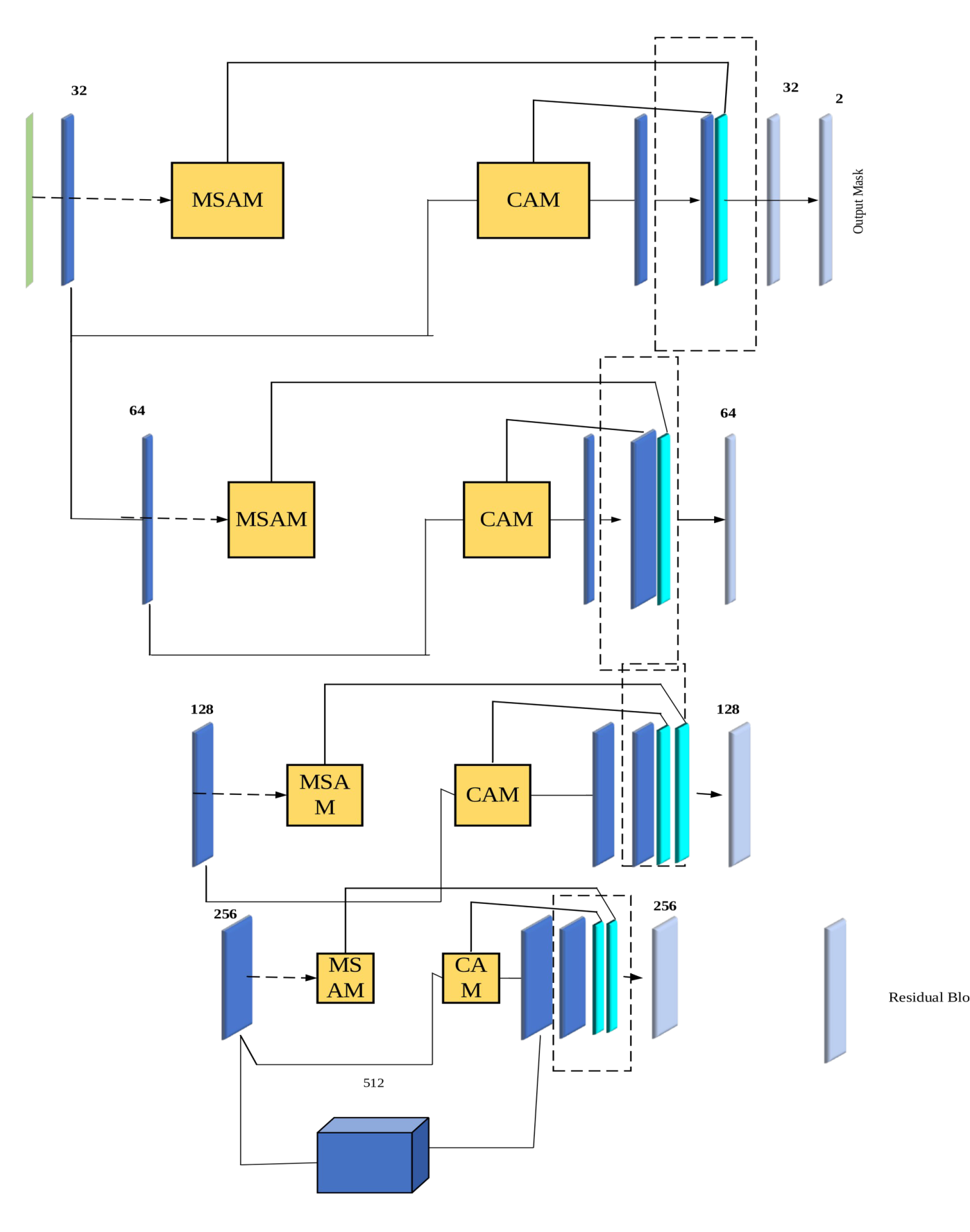
Figure 3: Model of multiscale dilated attention (MDA-Unet).

The expression for each residual unit is

Y_I=H(X_I)+f(X_I, w_I) (3)

X_I+1=f(Y_I) (4)

where X_I and X_I+1are the input and output of the I-th residual unit, respectively, and f(.) is the residual function f(Y_I) is the activation function, H(X_I) is an identity-mapping function. The weight vector for the I-th residual unit on the feature map is , w_I.

Multi-Scale Spatial Attention Module (MSAM) with Dilated Convolutions

The Multi-Scale Spatial Attention Module (MSAM) within your architecture harnesses the power of dilated convolutions to amplify spatial awareness and extend the receptive field. This is achieved by incorporating dilated convolutions within the MSAM module, strategically designed to capture spatial nuances across various scales. The magic lies in fine-tuning the dilation rate in these convolutions, which essentially acts as a zoom lens for the neural network. When the dilation rate varies, the network can adjust the scope of its view, gathering contextual information that is pivotal for accurate semantic segmentation. This is particularly evident when the MSAM module collaborates with the hybrid hierarchical dilated convolution module (HHDC), enabling the aggregation of spatial features from diverse spatial positions. In essence, dilated convolutions empower the MSAM to excel in tasks where understanding multi-scale context is paramount, such as semantic segmentation.

f_e^‘=m_s(f_e)⨂f_e (5)

Hybrid Hierarchical Dilated Convolution Module (HHDC) with Dilated Convolutions

Dilated convolutions serve as a cornerstone within the Hybrid Hierarchical Dilated Convolution (HHDC) module, strategically addressing the challenge of reduced feature resolution along the encoder path. Within HHDC, dilated convolutions play a pivotal role in rejuvenating the network’s receptive field and compensating for the feature loss incurred by max-pooling during encoding. This adaptive approach allows practitioners to finely adjust the dilation rate, thereby facilitating the capture of multi-scale contextual information. This flexibility proves especially beneficial for semantic segmentation tasks, where objects of diverse sizes must be accurately delineated. In essence, dilated convolutions represent a critical asset within the HHDC module, ensuring the preservation of contextual cues and significantly enhancing the quality of segmentation results by maintaining a comprehensive understanding of the visual scene.

Y=DilatedConv(x, 3×3,dilation_rate=2) (6)

Here Y is the dilated convolutional and x is the input. By adjusting the dilation rate, you can effectively capture multi-scale context information, which is essential for semantic segmentation, especially for objects of varying sizes. Dilated convolutions are a critical component of the HHDC module to maintain context information and enhance segmentation.

Channel Attention Module (CAM) with Skip Connections and Dilated Convolutions

The Channel Attention Module (CAM) represents a sophisticated fusion of skip connections and dilated convolutions, expertly tailored to elevate feature representation within the MDA-Unet model for semantic segmentation. Within CAM, dilated convolutions act as the spatial enhancers, capturing intricate spatial details and broadening the receptive field for improved context comprehension.

Simultaneously, skip connections bridge the original feature maps with their processed counterparts, promoting more comprehensive feature representation. This harmonious amalgamation of techniques empowers the model to excel at capturing nuanced context information while maintaining focus on crucial details. The channel attention mechanism, which operates on both encoder and decoder features in tandem, plays a pivotal role. By selectively attending to informative channels, it refines feature maps and optimizes model performance. These integrated components collectively address challenges related to gradient vanishing, context assimilation, and precise object segmentation, enhancing the overall efficacy of the MDA-Unet architecture for semantic segmentation tasks.

f_e^‘=m_C(f_e,f_D)⨂f_e (7)

The channel attention map is calculated as

m_C^e(f_e)=MLP(AvgPool(f_e))+MLP(MaxPool(f_e)) (8)

m_C^D(f_D)=MLP(AvgPool(f_D))+MLP(MaxPool(f_D)) (9)

m_C(f_e,f_D)=σ(m_C^e(f_e)+m_C^D(f_D)) (10)

The encoder and decoder features undergo element-wise summation after passing through their respective MLPs. Subsequently, the squeezed channel attention maps, denoted as m_C^e and m_C^D for element-wise summing fuses the decoder and encoder . Next, a sigmoid function is used to produce the final channel attention map, m_C(f_e,f_D).

Extraction of Features

In this research, Extraction of Features involves distilling significant attributes from segmented images. Color analysis reveals disease-specific color changes on crop leaves, with Color Space Transformations (e.g., RGB, HSV, LAB) aiding in identifying abnormal color patterns. Symmetry and regularity metrics like eccentricity detect irregularities in healthy leaf shapes. Texture features capture spatial intensity or color variances on the leaf surface, often indicative of diseases, utilizing techniques like Improved LrTP for precise texture analysis.

Color

Different diseases often manifest as distinct color changes on crop leaves. Color features can be extracted from images using techniques like Color Space Transformations (e.g., RGB, HSV, LAB). These features can help identify abnormal color patterns that indicate the presence of a disease.

Color Space Transformations

Converting colours from one representational foundation to another is referred to as colour space conversion. This frequently happens while translating a picture between colour spaces in order to maintain the original image’s resemblance while attaining accurate colour representation.

RGB

In the RGB color space, images are depicted as an m-by-n-by-3 numeric array, where elements define red, green, and blue channel intensity. The numeric value range varies with image data type, spanning [0, 1] for single or double arrays, effectively representing colors.

HSV

The HSV (Hue, Saturation, Value) colour space is a representation that differentiates an image for use in image processing colour information into hue, saturation, and value. Value denotes brightness, saturation denotes color intensity, and hue designates the predominant color tone. HSV offers advantages over typical RGB representation, notably in tasks like color-based object detection and segmentation, by providing a more accessible approach to handling and analysing color.

LAB

The Lab color space stands as a precise method for color representation, remaining independent of devices. This accuracy and portability render it applicable across diverse sectors, including printing, automotive, textiles, and plastics, owing to its ability to ensure consistent color depiction across various applications.

Symmetry and Regularity

Healthy leaves typically exhibit natural symmetry and regular patterning. Eccentricity is one metric that can be used to spot outliers and indicate abnormalities in their shapes and formations. This assessment assists in identifying possible irregularities and emphasizing potential symptoms of illness or stress that may be harming the development and plant’s growth

Eccentricity

Eccentricity measures the ratio of the focal distance to the major axis length of an ellipse in terms of symmetry and regularity. falling between 0 and 1, where 0 and 1 are unique circumstances. A circle has an eccentricity of 0, but a linear section has an eccentricity of 1, delineating the diverse forms an ellipse can encompass.

Texture

In feature extraction, texture features encapsulate the spatial disposition of intensity or color fluctuations on a leaf’s surface. Diseases frequently introduce distinct textures like spots, lesions, or patterns. To extract such intricacies, texture analysis employs methods such as the proposed Improved LrTP (Local ternary pattern) and features grounded in Local Quantized Texture (LQT), enabling precise disease identification through texture-based analysis.

Improved LrTP

Adaptive Manhattan Local Ternary Pattern

In the context of Local Ternary Patterns (LTP), the Adaptive Scaling Factor (α) plays a pivotal role and is meticulously fine-tuned through a novel hybrid optimization model. This model ensures that α is optimized for the specific task at hand. LTP measures the similarity between the central pixel (i, j) and its neighboring pixels within the defined neighborhood using the Manhattan distance metric. This approach enables robust and adaptive feature extraction by considering local patterns while also allowing for tailored scaling to enhance its effectiveness in various image analysis tasks. In the context of LTP, the limitation lies in its lack of gray-level transformation invariance, primarily due to the use of a fixed threshold, τ, across all neighborhoods. To address this, we introduce an innovative approach. Given a neighborhood ω(I,J) centered at pixel (I,J), with P_IJ representing the pixel’s gray value and μi,j denoting the average gray value of ω(I,J) we propose an adaptive threshold τ_IJ. This threshold is dynamically determined as τ_IJ=μ_IJ , allowing for tailored thresholding in each neighborhood, enhancing robustness to gray-level variations.

τ_IJ=⌊α×μ_IJ⌋ (11)

Manhattan Distance =|X1-X2|+|Y1-Y2| (12)

The scaling factor α modifies μ_IJ according to which the typical grey value in ω(I,J).

μ_IJ=(1)/(p+1)(P_i,J+∑_K=0^p-1(P_K)) (13)

The dynamic adaptation of threshold τ_IJ according to the gray-level variations within the neighborhood ω(I,J) is a key strategy for maintaining invariance to illumination transformations in the Manhottan Local Thresholding Process (MLTP). This dynamic thresholding approach enhances MLTP’s robustness to varying lighting conditions.

MLTP_p,r,τIJ=∑_K=0^p-1((P_K-P_I,J)×3^K, S(X)={1 X≥τ_IJ ; 0 |X|<τ_IJ ; -1 X≤-τ_IJ) (14)

The user-defined threshold, τ, remains a crucial parameter in the process. To address feature dimension reduction, This method separates each ternary pattern into its positive and negative portions, as seen in Figure 4. Although LTP codes exhibit enhanced noise resistance, they lose strict gray-level transformation invariance due to τ’s constant use across, when features are extracted from the database, all neighborhoods and images.

Soft concave -convex partition

In addressing the issue of neighborhoods having the same binary code in LBP-based operators but with different visual perceptions, a solution called Concave-Convex Partition (CCP) was introduced. CCP categorized neighborhoods into concave and convex groups based on a threshold, μ, representing the average gray value of the entire image. However, this approach’s rigidity stemmed from its dependency on a single threshold, μ, for classification.

To overcome this limitation, we introduce a more flexible approach known as Soft Concave-Convex Partition (SCCP). By introducing a scaling factor, β, SCCP allows for nuanced classification. If μ_I,J<(1-β)×μ, the central pixel (I,J) and its neighborhood ω(I, J) are classified as concave. Conversely, if μ_I,J≥(1+β)×μ, they are regarded as convex. When β = 0, SCCP simplifies to CCP, offering a continuum of partitioning choices to suit various image characteristics.

Based on SCCP, Orthogonal Combination of Adaptive Manhattan Local Ternary Pattern

In the research paper, a novel method named the Orthogonal Combination of Local Ternary Patterns is introduced, building upon OC_LBP and LTP. Figure 3 provides an illustrative example of the calculation process for an eight-pixel neighborhood. This OC_LTP approach is further enhanced by incorporating Manhottan Local Thresholding Process (MLTP) and Soft Concave-Convex Partition, resulting in the innovative Soft Concave-Convex Orthogonal Combination of Manhattan Local Ternary Patterns. A comparison of the dimensionality of the OC_MLTP,   SCC_OC_LTP,OC_LBP and is provided in Table 1. showcasing the advancements in feature extraction techniques.

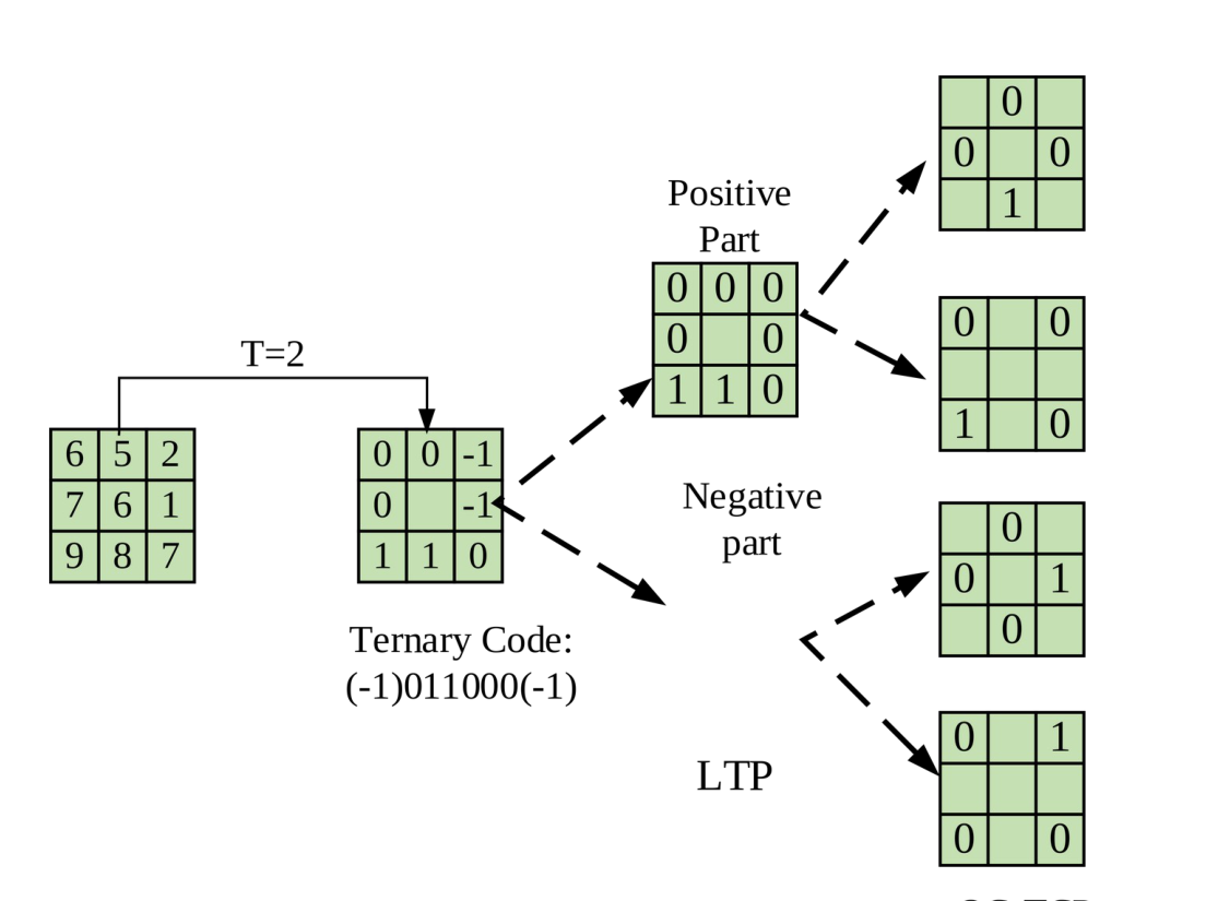
Figure 4 : The OC_LTP operators are calculated using eight nearby pixels.

Feature Selection

In this research, the feature is selected by using the Mountain Gazelle Optimizer (MGO) and the Marine Predator Algorithm (MPA) as part of the proposed hybrid optimization strategy to choose the most pertinent features. The focus is narrowed on discriminative characteristics as a result of the dimensionality reduction stage.

Hybrid Optimization (Marine Predator Algorithm+Mountain Gazelle Optimization)

Like many other metaheuristic algorithms, the Metaheuristic Population Algorithm is fundamentally a population-based technique. It begins by uniformly distributing the initial solution candidates across the entire search space during the first trial. This strategic approach forms the foundation for MPA’s exploration and optimization process.

x₀=x_min+rand(x_max-x_min) (15)

Utilizing lower bound x_minand upper bound x_max for variables, the formula incorporates a random vector (rand) that is uniform and falls between [0, 1].

Initialization

Drawing inspiration from a survival of the fittest environment, the dominant predator is the fittest individual and forms an Elite matrix. This matrix guides the search for prey by storing their positions.

Elite=[[x_1,1ⁱ , x_1,2ⁱ , ⋯ , x_1,Dⁱ] ; [x_2,1ⁱ , x_2,2ⁱ , ⋯ , x_2,Dⁱ] ; [⋮ , ⋮ , ⋮ , ⋮] ; [⋮ , ⋮ , ⋮ , ⋮] ; [⋮ , ⋮ , ⋮ , ⋮] ; [x_n,1ⁱ , x_n,2ⁱ , ⋯ , x_N,Dⁱ]]_N×D (16)

x⃗ⁱrepresents the Elite matrix, where n is the number of search agents, as well as is repeated n times to represent the top predator, and d denotes the dimensionality of the problem. This setup treats both predators and prey as search agents because, while predators seek their prey, the latter also search for their sustenance. After each iteration, the Elite matrix updates if the top predator is replaced by a more formidable predator. Another matrix, Prey, of the same dimension as Elite, guides predators in updating their positions. Essentially, the fittest prey (predator) initializes the Elite matrix.

Prey=[[x_1,1 , x_1,2 , ⋯ , x_1,D] ; [x_2,1 , x_2,2 , ⋯ , x_2,D] ; [x_3,1 , x_3,2 , ⋯ , x_3,D] ; [⋮ , ⋮ , ⋮ , ⋮] ; [⋮ , ⋮ , ⋮ , ⋮] ; [x_n,1 , x_n,2 , ⋯ , x_N,D]]_N×D (17)

Equation (17) utilizes Xi,j to represent the jth dimension of the ith prey, emphasizing the crucial role of these matrices in the optimization processFitness calculation

Fitness is calculated by the following formula

fit=min((E)) (18)

Where E is the error, Based on the fitness split the population as Territorial solitary Male(TSM) , Maternity Herd(MH), Bachelor Male Herds(BMH)

Territorial Solitary Males

Equation (19) mathematically depicts how adult male gazelles safeguard their territories from intruders, characterizing the behavior of Territorial Solitary Males (TSM)..

TSM=male_gazelle=|(RI₁×BH-RI₂×x(T))×f|×Cof_R (19)

Here, RI₁ and RI₂ represent random integers of 1 or 2, and malegazelle denotes the position vector of the most successful male gazelle observed. Equations (20), (21), and (22) are employed to calculate the values of BH, f, and Cof_R.

BH=x_Ra×R₁+m_PR×R₂ Ra={(n)/(3),………n} (20)

x_Rarepresents a random young male gazelle’s location within range Ra, while Mpr is the mean of search agents. n stands for the gazelle count, with R₁ and R₂ being random values in the (0, 1) range.

f=n₁(d)×exp((2-Iter×((2)/(MaxIter)))) (21)

The size of the problem dimension is expressed by n₁, and it is determined by a standard distribution. The Iter and MaxIter variables each denote the number of iterations and the most iterations possible.

Cof_I={(A+1)+R₃ ; A×n₂(d) ; R₄(d) ; n₃(d)×n₄(d)²×cos⁡((R₄×2)×n₃(d)) (22)

where r3 and r4 indicate for random numbers between 0 and 1.

At each iteration, a is calculated using Equation (23) based on n₂, n₃, and n₄, which are randomly generated values of the problem’s size.

A=-1+Iter×((-1)/(MaxIter)) (23)

Maternity Herd(MH)

Equation (24) illustrates a mathematical illustration of the reasoning that goes into a mother gazelle’s decision to defend its young.

MH=(BH+Cof_I,R)+(RI₃×male_gazelle-RI₄×x_rand)×Cof_I,R (24)

Where; x_randindicates the position in space of a gazelle selected at random from the population.

Integers RI₃ and RI₄ are chosen at random from (1, 2).

Bachelor Male Herds(BMH)

Young adult male gazelles establish their territories and attempt to get female gazelles to join them as a part of the maturation process for male gazelles. Equation (25) models this behavior.

BMH=(x(T)-d)+(RI₅×male_gazelle-RI₆×BH)×Cof_R (25)

Where x(T): is the gazelle’s position vector for the current iteration. The integers RI₅and RI₆are selected at random from (1, 2). R₆: is a value randomly selected from the range (0 1). Equation (26) is used to determine the value of d.

d=||x(T)+male_gazella||×(2×R₆-1) (26)

Migration in search of Food

Equation (27) models the random roaming behavior of mountain gazelles as they search for their preferred green pastures during foraging.

MSF=(ub-lb)×r₇+lb (27)

Bachelor Male Herds (BMH): Select the top 25% of solutions with the highest fitness values.
Maternity Herds (MH): Select the next 25% of solutions in terms of fitness.
Territorial and Solitary Males (TSM): Select the next 25% of solutions.
Migration Pattern in Search of Food (MSF): Select the remaining 25% of solutions.
Implement predator-prey behavior within each fitness-based group based on the velocity ratios specified in the three phases:

Phase 1

when the velocity ratio is high or when the predator is moving faster than the prey. In the early optimisation stages, where exploration is important, this scenario occurs. The optimum strategy for a predator in a high-velocity ratio (v=10) is to stay still, according to the criteria extrapolated. The following is how this rule’s mathematical model is used:

While Iter<(1)/(3)Max_Iter (28)

Stepsize⃗_I= r⃗_b ⊗(Elite⃗_I-r⃗_b⊗Prey⃗_I) I=1,….N (29)

Prey⃗_I=Prey⃗_I+p.r⃗ ⨂Stepsize⃗_I (30)

In the context of this scenario, RB, a vector with values drawn from a Normal distribution, is utilized for Brownian motion simulation through element-wise multiplication with the prey vector. The parameter P, set at 0.5, remains constant, and a vector of uniformly random numbers between [0,1] is represented by R. In the first third of iterations, when there is a strong potential for exploration because of a larger step size or velocity, this situation frequently arises. The words “Iter” and “Max_iter” stand for the current iteration with their respective maximum iteration limits.

Phase 2

Phase 2 represents a scenario where the predator and prey move at a balanced pace, resembling a hunt. This phase balances exploitation and exploration in the middle of optimization. Half the population focuses on each. Prey drives exploitation through Lévy movement, while predators use Brownian motion, optimizing their strategy for a unit velocity ratio (v ≈ 1).

while(1)/(3)MaxIter<Iter<(2)/(3)Max-Iter (31)

Population first half represents

Stepsize⃗_I= r⃗_l ⊗(Elite⃗_I-r⃗_l⊗Prey⃗_I) I=1,….N/2 (32)

Prey⃗_I=Prey⃗_I+p.r⃗ ⨂Stepsize⃗_I (33)

The research makes a different assumption for the second half of the population. Modeling Lévy movement for prey, RL is a vector of random numbers taken from the Lévy distribution. It simulates the prey’s movement by multiplying RL with Prey and adding the step size to the prey’s position. This predominantly involves small steps, enhancing exploitation during this phase.

Stepsize⃗_I= r⃗_b ⊗(r⃗_b⊗Elite⃗_I-Prey⃗_I) I=N/2,….N (34)

Prey⃗_I=Elite⃗_I+p.CF ⨂Stepsize⃗_I (35)

While CF=(1-(Iter)/(MaxIter))^{(2(Iter)/(MaxIter))}

The step size for predator movement is adjusted by an adjustable parameter. The prey adjusts its position in response to the predator’s Brownian movement, which is reproduced by multiplying RB by the Elite. This dynamic interaction guides the optimization process.

Phase 3

Phase 3 occurs during the optimisation process’s final stage when the predator outpaces the prey, emphasizing strong exploitation potential. The predator’s best course of action is Lévy movement with a low velocity ratio (v = 0.1). This phase prioritizes exploitation and marks the closing stages of the optimization process.

While Iter > 2/3 MAxIter

Stepsize⃗_I= r⃗_l ⊗(r⃗_l⊗Elite⃗_I-Prey⃗_I) I=1,….N (36)

Prey⃗_I=Prey⃗_I+p.CF ⨂Stepsize⃗_I (37)

In the Lévy strategy, adding the step size to the Elite position simulates the predator’s movement while multiplying r⃗_l and Elite replicates the predator’s movement to help update the position of the prey.

Effect of Eddy Formation and FADs

Incorporate the concept of eddy formation and FADs’ effect into the optimization process using Equation (38). This should apply to all groups

Prey⃗_I={Prey⃗_I +CF[x⃗_min+r⃗ ⨂(x⃗_max-x⃗_min)]⨂u⃗ if R≤FADs ; Prey⃗_I+[FADs(1-R)+R](Prey⃗_R1-(Prey⃗_R1)if R>FADs (38)

The probability that FADs will have an impact on optimisation is indicated by the parameter FADs = 0.2. The binary vector U formed by transforming random values in [0,1] to 0 if array is less than 0.2, else 1. r represents a uniform random number in [0,1]. x⃗_max and x⃗_min contain dimension boundaries. Subscripts R1 and R2 denote random indexes in the prey matrix.

Memory of the Marines

Implement marine memory by comparing the similarity of each current iteration’s solutions to their equivalents from the preceding iteration. If the current solution is more fit, replace the previous one. This should be applied to all groups.

Iteration Update

Continue with the iterations of the algorithm, updating the positions of solutions, adapting behaviors, and categorizing fitness until a termination condition is met.

VersaNet Deep Learning

Through the introduction of the VersaNet (proposed) deep learning paradigm, this research merges the LeNet, modified RNN, and EfficientNet frameworks, resulting in elevated performance and efficiency.

LeNet

LeNet (LeNet-5) is divided into two major components: a dense block made up of three fully linked layers and a convolutional encoder made up of two convolutional layers.

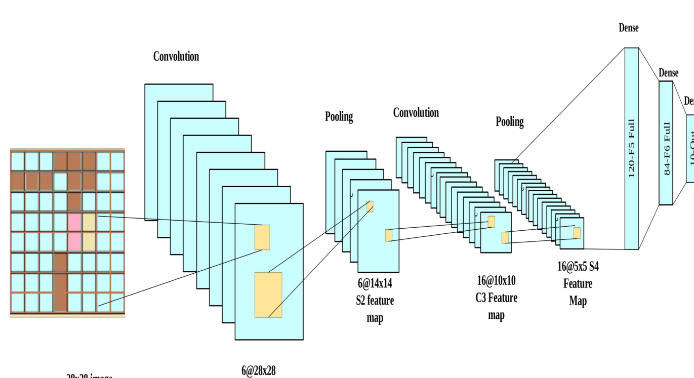
Figure 3: Architecture of LeNet

Within every convolutional block, the fundamental components encompass Sigmoid activation function, convolutional layer, and average pooling procedure are applied. It’s interesting to observe that despite having better performance, ReLUs and max-pooling have not yet been fully explored. A kernel and a sigmoid activation are used in each convolutional layer to direct spatially organized inputs into two-dimensional feature maps with larger channel dimensions. 6 output channels are created by the first convolutional layer, whereas 16 are produced by the second. Employing pooling operations , dimensionality reduction transpires, downsizing spatial features by a specific factor. Consequently, the convolutional block issues output with dimensions shaped as (batch size, channel count, height, and width).

For transitioning it is essential to flatten each instance in the minibatch before it is output from the convolutional block to the dense block. This four-dimensional input is essentially converted into the desired two-dimensional arrangement, suitable for fully connected layers’ needs. Recall that the ideal two-dimensional representation uses the first dimension to index minibatch examples and the second to configure a flat vector portrayal for each sample. Three fully connected layers make up the thick block of LeNet, and each of them produces 120, 84, and 10 outputs, respectively.

Recurrent Neural Networks

Recurrent neural networks were developed primarily to overcome the limitations of feedforward neural networks for simulating sequences. RNN networks are made up of neurons or component parts that have the potential to recall past observations. This makes it possible for RNNs to model the input data using observations made both recently and in the past. One of the suggested RNNs, the Long Short-Term Memory (LSTM) architecture, excelled in simulating the long-range temporal dependencies of the input data. Given an input vector a(s) and the current observation (let’s say a(s+1)), the LSTM unit formally performs the following operations in recursive fashion:

Recurrent neural networks (RNNs) were designed specifically to get around the challenges of feedforward neural networks in handling sequence data. Comprising neurons with memory components, RNNs can effectively learn from past observations, accommodating both recent and distant information. Among recommended RNN variants, the Long Short-Term Memory architecture excels in capturing intricate long-range temporal dependencies within input data. In a formal context, the LSTM unit iteratively conducts operations using an input vector A(S) and the current observation a(S+1), making it adept at modeling sequences with complex temporal relationships, like natural language and time series data.

J(S)=σ[b_D[a(S),G(S-1)+W_J]] (25)

D̅(S)=tanh([B_D[a(S),G(S-1)]+W_D]) (26)

U(S)=σ(b_U[a(S)[A(S),G(S-1)]+W_U] (27)

D(S)=U(S)ʘ D(S-1)+ J(S) ʘ d̅(S) (28)

p(S)=σ[b_P[a(S),G(S-1)]+W_P] (29)

G(S)=PS ʘtanh((D(S))) (30)

where ʘ is the matrix multiplication done element-by-element. While J,U,D ,p are collectively known as input, input modulation, forget, cell, and output gates and carry out operations that enable the LSTM to choose the information to remember and to forget from the incoming data, b_J, b_D,b_U, b_P and W_J,W_D, W_U,W_P learnable kernels and biases, respectively. When combined with A, the hidden state G encodes the information that the LSTM unit has learned from prior observations.

Efficient Net

EfficientNet stands as a method for designing as well as scaling convolutional neural networks that reliably modifies the depth, breadth, and resolution parameters using a composite coefficient. EfficientNet takes a unique approach by uniformly adjusting depth, width, and resolution—representing layers, channels, and image size—yielding enhanced performance while maintaining architectural cohesion and reducing parameters. Scaling each dimension employs predetermined scaling coefficients, computed methodically. The process involves an optimal coefficient determination through grid search. This systematic exploration establishes the correlation between distinct network dimensions within predefined constraints, such as doubling FLOPS. The outcome is an architecture that maximizes efficiency, optimizing each element’s contribution and effectively improving network capabilities.

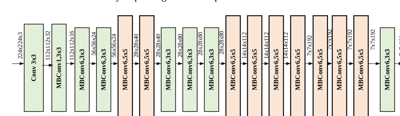
Figure 4: Basic architecture of EfficientNet

Employing the Mobile Inverted Convolution (MBConv) technique, also known as Inverted Residual Block, this architecture utilizes an inventive inverted structure. This involves sum-product operations, skip connections in narrow regions, and channel reduction, while retaining the initial channel count. The MBConv follows a narrow-wide-narrow design strategy, divergent from traditional Convolutional networks. It widens via a 1×1 Convolution, employs a 3×3 Depth-wise Convolution for parameter reduction, and further compresses channels with a subsequent 1×1 Convolution. The EfficientNet-B7 model excels in scaling dimensions while maintaining high accuracy per parameter, ultimately yielding a compact yet accurate architecture.

Result and Discussion

Experimental Setup

The suggested model is trained with Improved LrTP to achieve excellent performance in detecting crop leaf diseases. The accuracy, precision, recall, F-Measure, sensitivity, FPR, FNR, and specificity metrics were used to find out the performance of the model.

Performance overall of the proposed model

In this research , identifying agricultural leaf diseases, the proposed model has proven to perform exceptionally well. Numerous performance indicators, such as  Precision, Accuracy, F-Measure, Recall, False Positive Rate, Sensitivity, Specificity and  False Negative Rate (FNR)., were meticulously employed to assess its capabilities. In Table 2, With an outstanding accuracy of 96.19%, the proposed model showcases its prowess in accurately categorizing instances of crop diseases, a crucial factor in agricultural decision-making. Its precision score of 96.06% reflects its ability to minimize false positive identifications, thereby reducing unnecessary interventions in healthy crops. An impressive recall rate of 95.84% highlights the model’s adeptness at identifying genuine cases of crop leaf diseases, ensuring minimal instances of false negatives. The F-Measure merges recall and precision  into one statistic stands remarkably high at 95.95%, underscoring the well-rounded performance of the model. Sensitivity, a measure of the true positive rate, further attests to its effectiveness in correctly flagging diseased crops. Moreover, the model exhibits exceptional specificity at 99.82%, indicating its aptitude for accurately discerning healthy crops. The low False Positive Rate (FPR) of just 0.18% minimizes the chances of erroneously classifying a healthy crop as diseased, while the equally low False Negative Rate (FNR) of 4.16% ensures that actual instances of crop diseases are rarely overlooked. While other models like LeNet, RNN, and EfficientNet perform respectably, the proposed model, fortified by Improved LrTP, emerges as a robust and dependable tool for crop disease detection, holding significant promise for advancing agricultural practices and safeguarding crop yields.

Table 2: Overall Performance of the metrics of the proposed model

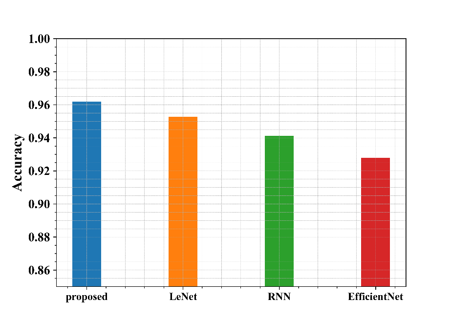
Figure 5: Graphical format of the Accuracy metrics of the proposed model with other comparitive model

From Fig. 5 it clearly illustratess the suggested model has greater accuracy metrics than other comparable models like LeNet,RNN, EfficientNet.

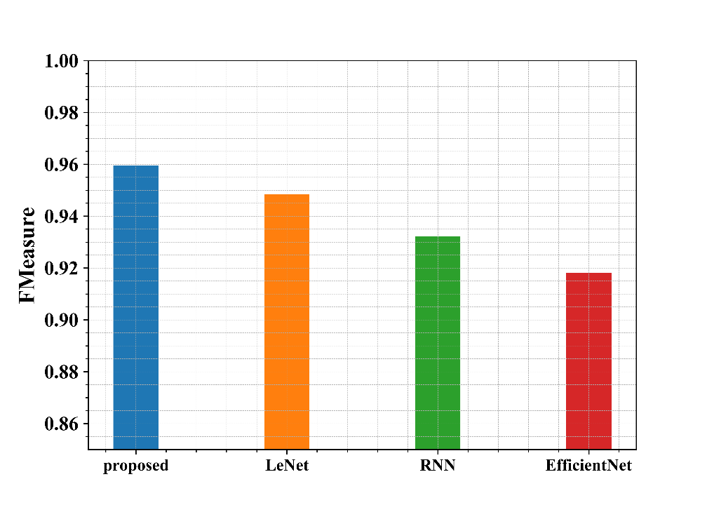
Figure 6: Analysis of the proposed model’s F-Measure measures’ performance in comparison to other models, represented graphically

Figure 6 illustrates that the F-Measure Metrics of the suggested model is higher than the other comparitive models like LeNet, RNN, EfficientNet.

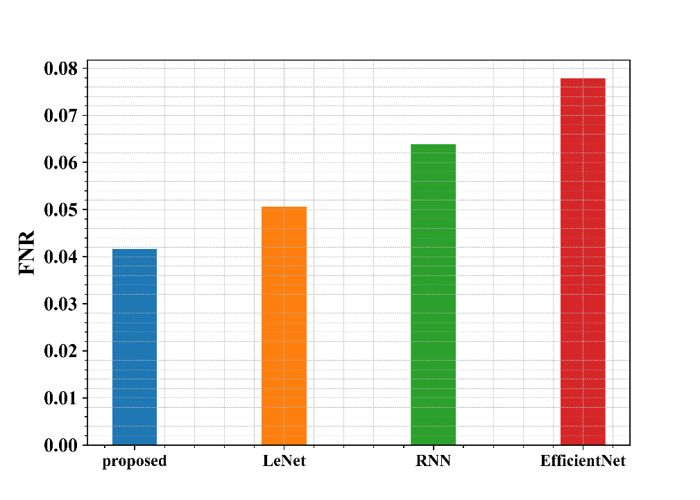
Figure 7: Performance analysis of the FNR metrics of the proposed model with other comparitive model graphical representation

Figure 7 illustrates that the FNR Metrics of the suggested model is lower than the other comparitive models like LeNet, RNN, EfficientNet.

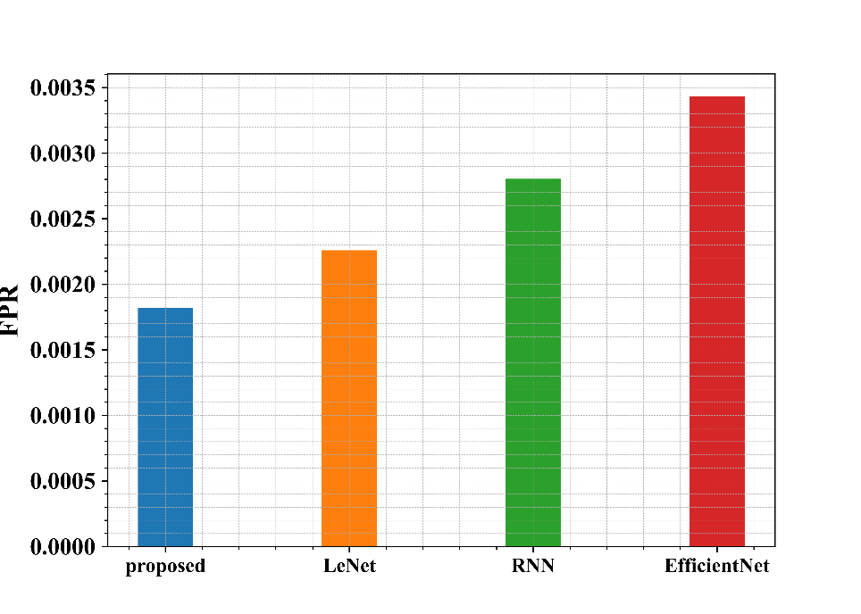
Figure 8: Performance analysis of the FPR metrics of the suggested model with other comparitive model graphical representation

From Fig. 8 it illustrates that the FPR Metrics of the proposed model is lower than the other comparitive models like LeNet, RNN, EfficientNet.

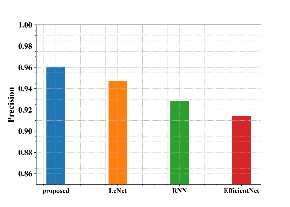
Figure 9: Performance analysis of the Precision metrics of the suggested model with other comparative model graphical representation

Figure 9 illustrates that the Precision Metrics of the proposed model is higher than the other comparitive models like LeNet, RNN, EfficientNet.

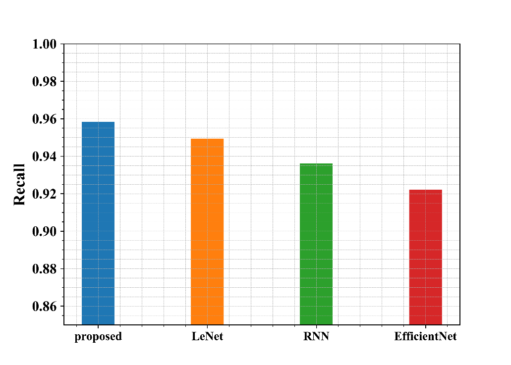
Figure 10: Performance analysis of the Recall metrics of he proposed model in comparison to other models graphical representation

From Figure 10, the Recall Metrics of the suggested model clearly show that they are greater than those of the other comparative models like LeNet, RNN, EfficientNet.

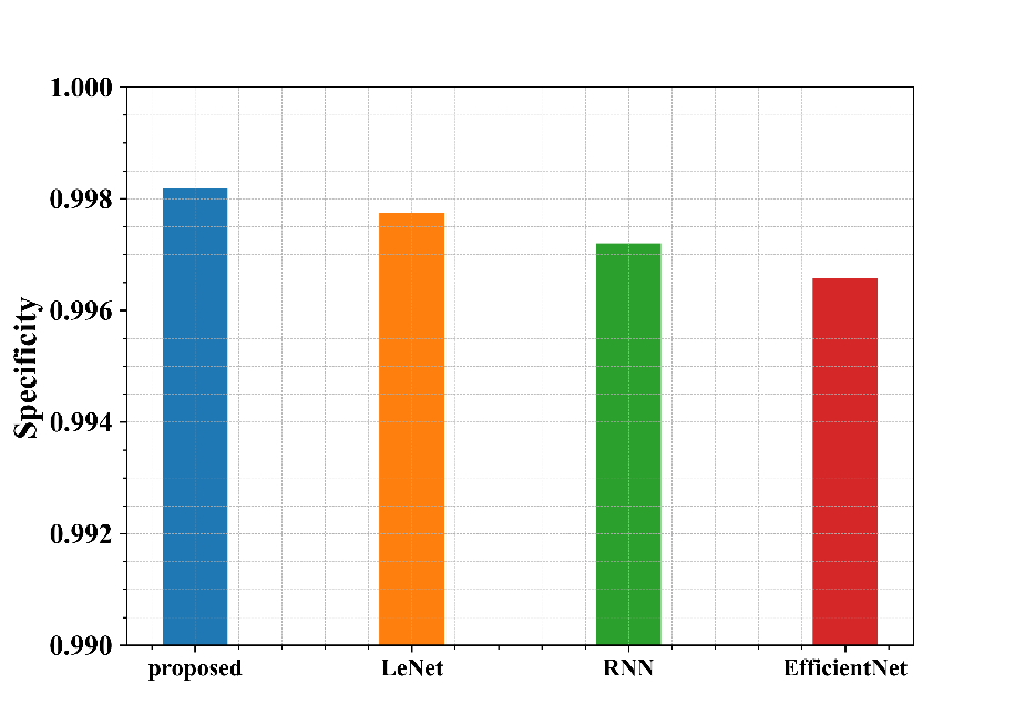
Figure 11: Performance analysis of the Specificity metrics of the suggested model with other comparative model graphical representation

Figure 11 illustrates that the specificity metrics of the suggested model is higher than the other comparitive models like LeNet, RNN, EfficientNet.

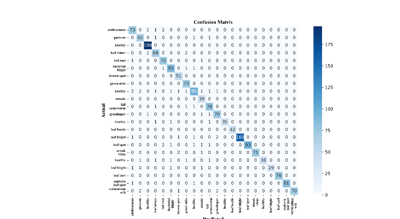
Figure 12: Confusion Matrix

Figure 12 provides a visualization of the Confusion Matrix, offering by comparing the model’s performance to the actual and projected results as well as classifying cases into true positives, true negatives, false positives, and false negatives, one can obtain a thorough and organized depiction of the model’s performance. This matrix is an important tool for evaluating the categorization of the model. accuracy and error rates.

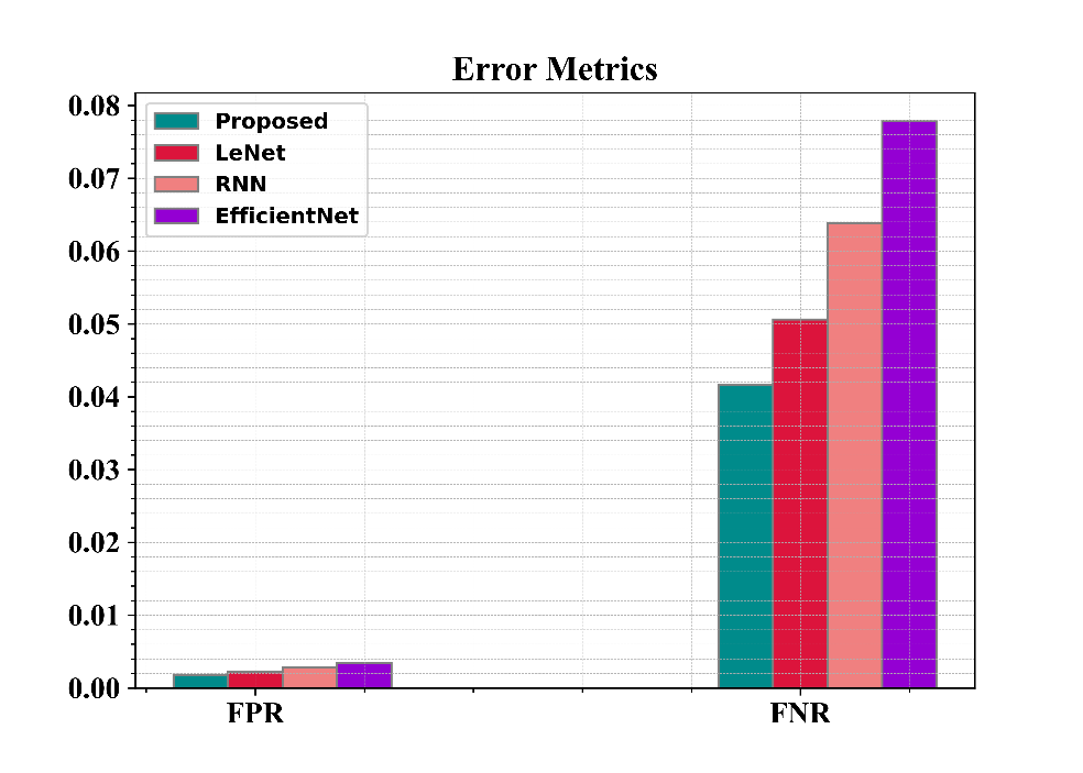
Figure 13: Error Metrics

Figure 13 illustrates the error metrics, presenting a concise and informative graphical representation of key performance indicators such as FPR and FNR. This visual aid is instrumental in assessing the model’s overall effectiveness and its ability to balance FPR and FNR in classification tasks.

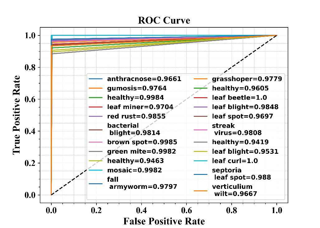
Figure 14 :ROC Curve

Figure 14 showcases the ROC Curve, a graphical illustration that evaluates performance of the model in separating true positives and false positives over various threshold levels. This curve offers insightful information about the model’s capacity to balance genuine positives and false positives, aiding in threshold selection for optimal classification results.

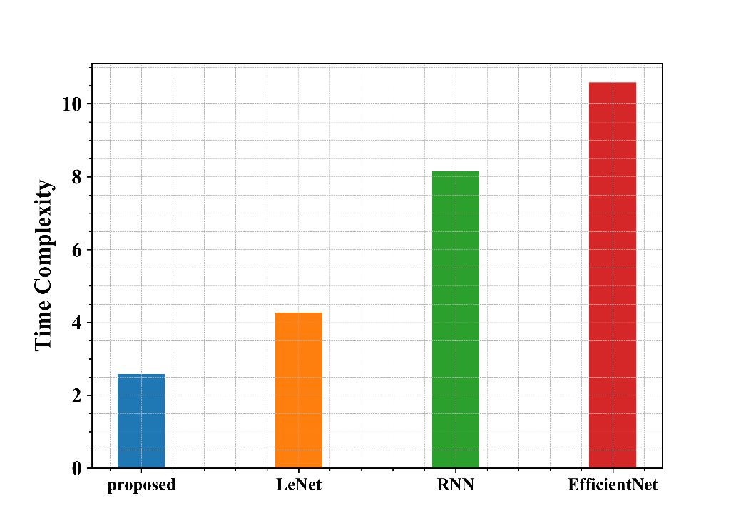
Figure 15: Graphical Representation of Time Complexity of the proposed model

Fig .15, Illustrates the graphical format of the time complexity between the proposed and the other comparative models ,it is clearly noticed that the time complexity of the proposed model is lowel than the other comparativ models.

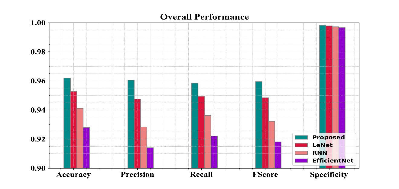
Figure 16: Graphical Representation of the Overall Performance of the proposed model

Figure 16 illustrates the overall performance metrics like Recall, F-score, Accuracy, Precision, as well as Specificity. The figure it is clearly explained that the proposed model performance metrics accuracy, Recall, F-score, Specificity, and Precision are higher than that of the other models.

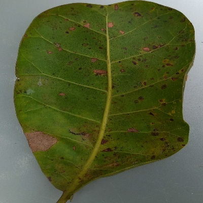
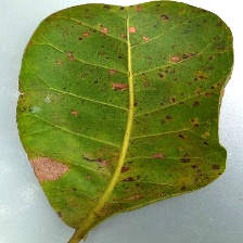
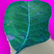
Figure 17: Images of Original, Preprocessed and the Segmented

Figure 17 shows three images, each serving a specific function: the Original Image, displaying the raw data or input; the Preprocessed Image, showing the data after any necessary improvements or cleaning; and the Segmented Image, displaying the data after splitting or grouping for analysis.

Conclusion

In conclusion, our detailed methodology for precise leaf disease detection stands as a pivotal advancement in addressing the profound challenges that crop leaf diseases pose to agricultural productivity. By seamlessly integrating cutting-edge techniques in image processing, segmentation, feature extraction, and deep learning, we have crafted a powerful solution for accurate and versatile disease identification within agricultural contexts. Our journey begins with meticulous image pre-processing, laying the foundation for robust analysis through data augmentation, normalization, color enhancement, and noise reduction. We then employ Semantic Segmentation, harnessing the capabilities of the Architecture for U-Net using skip connections and dilated convolutions to precisely delineate disease-affected regions. Feature extraction spans various dimensions, from color patterns to symmetry, regularity metrics, and complex textures. The subsequent feature selection, guided by a hybrid optimization approach, refines our focus on the most discriminative characteristics. At its core, our methodology introduces the innovative VersaNet deep learning framework, which combines the strengths of LeNet, RNN, and EfficientNet. This fusion empowers the model to comprehend diverse data modalities effectively. Implemented in Python, our approach has been rigorously validated on real-world crop datasets, affirming its efficacy. By enabling proactive disease management in agriculture, our methodology contributes to the broader goal of enhancing crop yield and global food security. Its versatility and precision make it a valuable asset for farmers and researchers alike in the ongoing battle against crop leaf diseases.

References

Sujatha, R., Chatterjee, J.M., Jhanjhi, N.Z. and Brohi, S.N., 2021. Performance of deep learning vs machine learning in plant leaf disease detection. Microprocessors and Microsystems, 80, p.103615.

Ahmed, A.A. and Reddy, G.H., 2021. A mobile-based system for detecting plant leaf diseases using deep learning. AgriEngineering, 3(3), pp.478-493.

Yadav, S., Sengar, N., Singh, A., Singh, A. and Dutta, M.K., 2021. Identification of disease using deep learning and evaluation of bacteriosis in peach leaf. Ecological Informatics, 61, p.101247.

Xiong, Y., Liang, L., Wang, L., She, J. and Wu, M., 2020. Identification of cash crop diseases using automatic image segmentation algorithm and deep learning with expanded dataset. Computers and Electronics in Agriculture, 177, p.105712.

Trivedi, N.K., Gautam, V., Anand, A., Aljahdali, H.M., Villar, S.G., Anand, D., Goyal, N. and Kadry, S., 2021. Early detection and classification of tomato leaf disease using high-performance deep neural network. Sensors, 21(23), p.7987.

Zhou, C., Zhou, S., Xing, J. and Song, J., 2021. Tomato leaf disease identification by restructured deep residual dense network. IEEE Access, 9, pp.28822-28831.

Y. Zhang, C. Song and D. Zhang, “Deep Learning-Based Object Detection Improvement for Tomato Disease,” in IEEE Access, vol. 8, pp. 56607-56614, 2020, doi: 10.1109/ACCESS.2020.2982456.

Chowdhury, M.E., Rahman, T., Khandakar, A., Ayari, M.A., Khan, A.U., Khan, M.S., Al-Emadi, N., Reaz, M.B.I., Islam, M.T. and Ali, S.H.M., 2021. Automatic and reliable leaf disease detection using deep learning techniques. AgriEngineering, 3(2), pp.294-312.

Hernández, S. and López, J.L., 2020. Uncertainty quantification for plant disease detection using Bayesian deep learning. Applied Soft Computing, 96, p.106597.

Saleem, M.H., Khanchi, S., Potgieter, J. and Arif, K.M., 2020. Image-based plant disease identification by deep learning meta-architectures. Plants, 9(11), p.1451.

Coulibaly, S., Kamsu-Foguem, B., Kamissoko, D. and Traore, D., 2019. Deep neural networks with transfer learning in millet crop images. Computers in industry, 108, pp.115-120.

Barbedo, J.G.A., 2019. Plant disease identification from individual lesions and spots using deep learning. Biosystems engineering, 180, pp.96-107.

Khamparia, A., Saini, G., Gupta, D., Khanna, A., Tiwari, S. and de Albuquerque, V.H.C., 2020. Seasonal crops disease prediction and classification using deep convolutional encoder network. Circuits, Systems, and Signal Processing, 39, pp.818-836.

Vallabhajosyula, S., Sistla, V. and Kolli, V.K.K., 2022. Transfer learning-based deep ensemble neural network for plant leaf disease detection. Journal of Plant Diseases and Protection, 129(3), pp.545-558.

Lee, S.H., Goëau, H., Bonnet, P. and Joly, A., 2020. New perspectives on plant disease characterization based on deep learning. Computers and Electronics in Agriculture, 170, p.105220.

Anami, B.S., Malvade, N.N. and Palaiah, S., 2020. Deep learning approach for recognition and classification of yield affecting paddy crop stresses using field images. Artificial intelligence in agriculture, 4, pp.12-20.

Ai, Y., Sun, C., Tie, J. and Cai, X., 2020. Research on recognition model of crop diseases and insect pests based on deep learning in harsh environments. IEEE Access, 8, pp.171686-171693.

Chen, J., Chen, J., Zhang, D., Sun, Y. and Nanehkaran, Y.A., 2020. Using deep transfer learning for image-based plant disease identification. Computers and Electronics in Agriculture, 173, p.105393.

Tiwari, V., Joshi, R.C. and Dutta, M.K., 2021. Dense convolutional neural networks based multiclass plant disease detection and classification using leaf images. Ecological Informatics, 63, p.101289.

Sharma, P., Berwal, Y.P.S. and Ghai, W., 2020. Performance analysis of deep learning CNN models for disease detection in plants using image segmentation. Information Processing in Agriculture, 7(4), pp.566-574.

Nagasubramanian, K., Jones, S., Singh, A.K., Sarkar, S., Singh, A. and Ganapathysubramanian, B., 2019. Plant disease identification using explainable 3D deep learning on hyperspectral images. Plant methods, 15, pp.1-10.

Waheed, A., Goyal, M., Gupta, D., Khanna, A., Hassanien, A.E. and Pandey, H.M., 2020. An optimized dense convolutional neural network model for disease recognition and classification in corn leaf. Computers and Electronics in Agriculture, 175, p.105456.

Jiang, F., Lu, Y., Chen, Y., Cai, D. and Li, G., 2020. Image recognition of four rice leaf diseases based on deep learning and support vector machine. Computers and Electronics in Agriculture, 179, p.105824.

Zhao, Y., Liu, L., Xie, C., Wang, R., Wang, F., Bu, Y. and Zhang, S., 2020. An effective automatic system deployed in agricultural Internet of Things using Multi-Context Fusion Network towards crop disease recognition in the wild. Applied Soft Computing, 89, p.106128.

Arsenovic, M., Karanovic, M., Sladojevic, S., Anderla, A. and Stefanovic, D., 2019. Solving current limitations of deep learning based approaches for plant disease detection. Symmetry, 11(7), p.939.

Editorial Staff

Academic Master Education Team is a group of academic editors and subject specialists responsible for producing structured, research-backed essays across multiple disciplines. Each article is developed following Academic Master’s Editorial Policy and supported by credible academic references. The team ensures clarity, citation accuracy, and adherence to ethical academic writing standards

Content reviewed under Academic Master Editorial Policy.

• Editorial Staff

  Grid-Connected Solar PV Systems and Power Quality Review
• Editorial Staff

  Predicting Cardiovascular Diseases with PCA and Artificial Neural Networks
• Editorial Staff

  Maternal and Neonatal Outcomes Following Water Birth Systematic Review and Meta-Analysis
• Editorial Staff

  Electrospun Polymeric Nanofibers for Biomedical Applications