ChromoEnsembleNet for Chromosome Structure Detection

Abstract

This research proposes an advanced approach for accurate chromosome structure detection using deep learning techniques. uses sophisticated preprocessing techniques, including Bilateral filtering, to enhance image quality while effectively reducing noise in chromosome images. Harnessing the power of GANs, significantly augment the dataset by generating highly realistic synthetic chromosome images. This diversifies the dataset and enhances the model’s ability to detect various chromosome structures, introduce a novel optimized U-Net architecture for precise semantic segmentation, enabling accurate identification of critical chromosome regions and adopt transfer learning with pre-trained transformer models like Vision Transformer (ViT) to extract rich features, further complemented by shape, color, and texture-based descriptors, proposed hybrid optimization algorithm, a fusion of Dwarf mongoose and Prairie dog optimization, intelligently selects the most relevant and discriminative features, optimizing the feature space and reducing dimensionality. To ensure robust chromosome structure classification, present the ChromoEnsembleNet architecture approach combines the strengths of multiple classifiers, such as DenseNet, ResNet, EfficientNet, and Random Forest, using a voting mechanism to enhance feature reuse and gradient flow, ultimately achieving precise chromosome structure detection The proposed approach achieves precise chromosome structure detection, supporting early diagnosis and treatment of genetic disorders. The tool used is PYTHON. This research contributes to advancing medical imaging and genetic research, with the potential for improving patient care through accurate and efficient chromosome analysis. The experimental values are reported as supplied; the evaluation limitations discussed below restrict their interpretation.

Keywords: chromosome structure detection; Generative Adversarial Networks, U-Net, Region of Interest, Vision Transformers, Chromo Ensemble Net, Dwarf mongoose and Prairie dog optimization

Introduction

Chromosomes are cellular structures carrying DNA inside the cell’s nucleus, crucial for genetic information transmission. Innovative deep learning approach for chromosome defect detection, utilizing 20,299 images from Dongguan Kanghua Hospital, with feature fusion for accurate abnormality identification [1]. TPM and GVP induced considerable genotoxicity, causing up to six times more micronucleated cells and up to ten times more aberrant metaphases than the negative control [2]. Innovative study on deep learning for chromosome detection in metaphase images, featuring novel preprocessing and false positive/negative reduction. Evaluated using 74 images from the CRCN-NE database, with 2174 regions. Assessing segmentation, classification, and detection of chromosomes in original images [3]. Automating the selection of suitable metaphase chromosomes for genetic disorder analysis reduces manual effort and saves time [4]. Introducing Varifocal-Net, a novel deep learning approach for rapid karyotype diagnosis, simultaneously classifying chromosome type and polarity [5].

The presence of past male-mediated expansions in the genetic record can be explored through analysis of the Y chromosome’s male-specific region [6]. Introducing a proposed molecular architecture for human chromosome 10, derived from cryo-EM cellular tomography of interphase chromosomes [7]. Hi-C is an advanced method for comprehensive chromatin interaction detection in mammalian nuclei, using Chromosome Conformation Capture, crosslinking, digestion, and re-ligation of covalently linked DNA fragments [8]. Proposing an intrusion detection model using an enhanced genetic algorithm (GA) and deep belief network (DBN). The GA iteratively optimizes hidden layer numbers and neuron counts, achieving accurate detection with a compact structure [9]. To compare chromosomal microarray analysis (CMA) detection rate with conventional karyotype in prenatal fetuses. Additionally, it seeks to evaluate CMA’s diagnostic benefits in various indication groups [10].

Developing a method to identify threshold values for microtubule inhibitor-induced chromosome loss and non-disjunction is vital for risk assessment and the lack of accurate data on such thresholds, makes risk calculations challenging [11]. Existing methods using convolutional networks lack dropout layers and norm regularization to prevent overfitting. Suboptimal parameter settings hinder their performance [12]. Traditional karyotyping and microarrays are their limited resolution to identify small or hidden genetic changes, which are now more effectively revealed through advanced sequencing techniques. This motivates the use of genome sequencing in both research and clinical fields to gain a comprehensive understanding of genomic variations and their implications in various diseases and disorders [13]. A groundbreaking study utilizes 3D-CNN for brain MRI classification and introduces GABM for better interpretability, revolutionizing neuroimaging research [14]. Focus on deep neural network connectivity, introducing layer-wise structure learning via multi-objective optimization. Improved generalization by reducing connections overcomes overfitting, leading to efficient and effective models [15].

The document’s structure is as follows: Section 1 serves as the introduction, while Section 2 comprises a comprehensive literature review, detailing various methods used in prior research. Section 3 presents the proposed methodology. Research outcomes are discussed in Section 4, and Section 5 concludes the document.

Literature Review

In 2015, Rastegari and Hingston et al. [16] have introduced a GA-based approach for network intrusion detection, with high detection performance and interpretable rulesets. Comparing with non-GA algorithms (decision trees, rule induction, kNN) and GA-based methods (GASSIST-ADI, MPLCS). Our approach balances accuracy and understandability, overcoming the drawbacks of both conventional and complex GA-based techniques.

In 2020, Salle and Galateau et al. [17] have focused on in-depth characterization of the TM subtype through histological, immunohistochemical, and molecular analysis. Deep learning was utilized to analyze pathological slides in this cohort. The drawback of deep learning lies in the requirement for large amounts of labeled data for effective training, which may be challenging to obtain for rare subtypes. However, once trained, deep learning models can provide accurate and automated analysis, leading to significant advancements in cancer research and diagnosis.

In 2020, Chung and Shin et al. [18] have utilized multi-channel convolutional neural networks (CNNs) to predict stock index fluctuations. The network topology was optimized to enhance model performance. The drawback was the extensive hyper-parameter tuning required for constructing an efficient model for data pattern learning. Nonetheless, CNNs successfully captured complex features and provided accurate predictions in financial time series analysis.

In 2019, Qin and Wen et al. [19] have used the Varifocal-Net for chromosome classification, evaluated on a large dataset. It used a three-stage CNN-based method. In the first stage learned global and local features with G-Net and L-Net, respectively. The second stage utilized two MLP classifiers for robust differentiation. However, a drawback was the complexity in tuning hyperparameters during development. In the third stage, a dispatch strategy was employed based on predicted probabilities for chromosome type assignment. Overall, the Varifocal-Net demonstrated accurate chromosome classification with the potential for further optimization and efficiency improvements.

In 2020, Qiao and Zhu et al. [20] have proposed deep learning with CNNs and GPU acceleration for microaneurysm detection in fundus images. Utilizing semantic segmentation, it graded fundus images for diabetic retinopathy but required a large and diverse dataset for optimal performance. Once trained, the system efficiently assisted ophthalmologists in diagnosing diabetic retinopathy.

In 2019, Fang and Tan et al. [21] have suggested PPR-Meta, a 3-class classifier, effectively identified phages and plasmids in metagenomic data, addressing the lack of satisfactory existing tools. However, its drawback was the requirement for a large and diverse dataset for optimal training. Once trained, PPR-Meta significantly contributed to understanding microbial communities and their genetic elements in metagenomic assemblies.

In 2020, Kasani and Park et al. [22] have proposed an aggregated deep-learning model for Leukemic B-lymphoblast classification. Data augmentation addressed the limited dataset size, and transfer learning improved performance. However, careful selection and fine-tuning of transfer learning models were required. The model demonstrated reliable and accurate classification of Leukemic B-lymphoblasts, highlighting deep learning’s potential in medical diagnosis.

In 2018, Saha and Chakraborty et al. [23] have proposed automated mitosis detection in H&E-stained breast cancer histology images. Deep architecture, combined with handcrafted features from three challenges, significantly improved the performance of the deep learning framework. However, a drawback was the potential complexity of tuning hyperparameters for optimal results. The comparison results highlighted the strength and effectiveness of the proposed methodology.

In 2020, Hu and Maurais et al. [24] have developed various methods to interrogate human GCRs. These included cellular and genomic approaches with both clinical and experimental use. Advantages included discovering novel rearrangement types implicated in human disease, but drawbacks included technical limitations and the complexity of data interpretation. The combination of these approaches led to significant advances in understanding the mechanisms driving GCR formation.

In 2017, Sati and Cavalli et al. [25] have introduced significant advancements in biochemical approaches for mapping chromatin interactions. Technological improvements enhanced the general approach and provided valuable biological insights. Despite mentioning various 3C basic steps and their pitfalls, limitations included technical complexities and the need for sophisticated data analysis methods

Problem Statement

Table 1: Overview of the aim and drawbacks of the previous research

Proposed Methodology

Detecting chromosome structures using deep learning is a critical task in medical image analysis. Accurate identification of chromosomal abnormalities can aid in the early diagnosis and treatment of genetic disorders. In this research work, propose an advanced approach for detecting chromosome structures using deep learning techniques, with a focus on enhancing the quality of input images, augmenting the dataset, and efficiently extracting informative features. The Overall flow diagram is depicted in Fig 1.

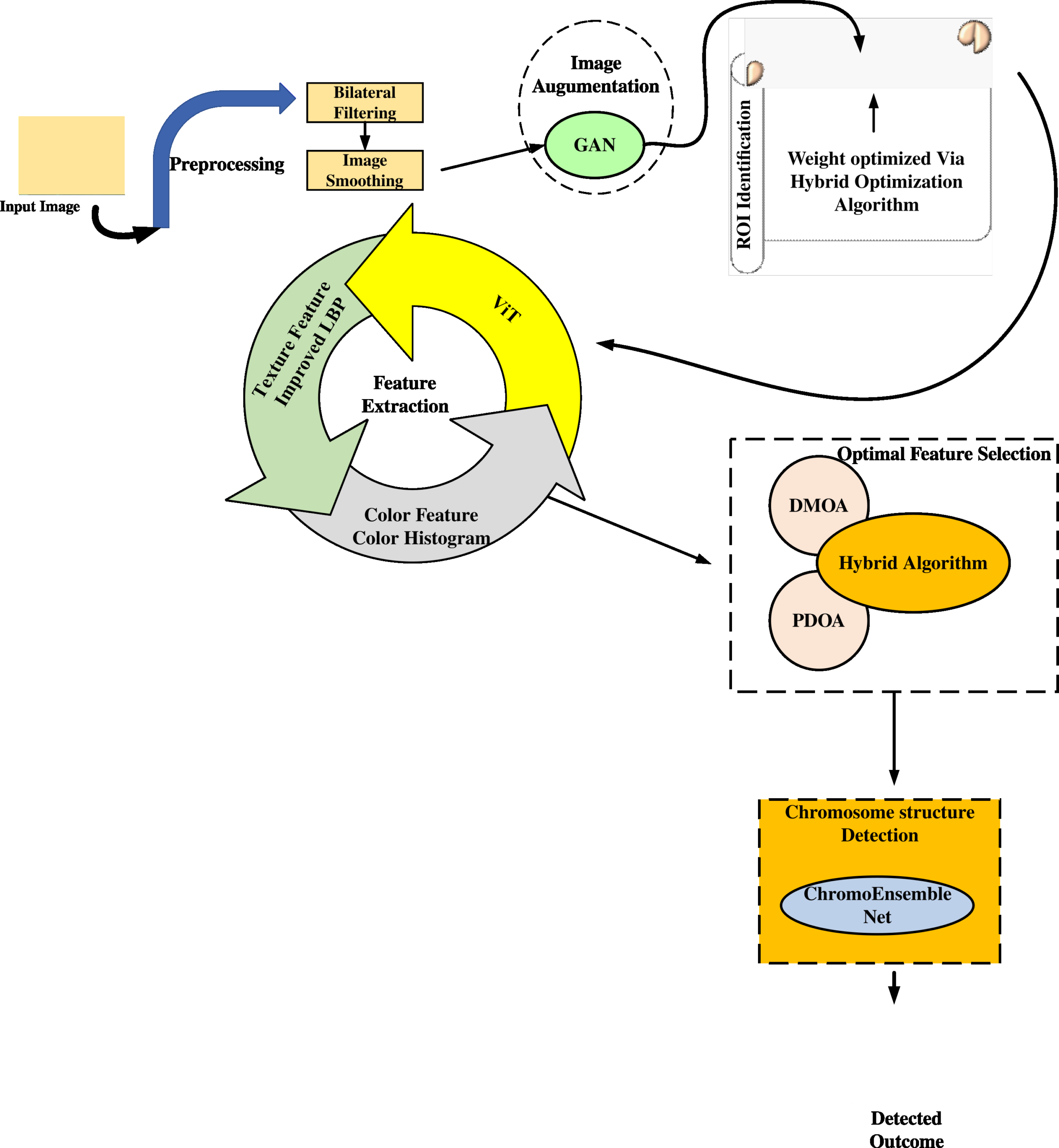
Figure 1: Overall Flow diagram of the proposed model

Pre-processing

In this research, the chromosome images undergo advanced preprocessing to enhance image quality and reduce noise effectively. The chromosome images undergo filtering and image smoothing techniques to enhance image quality and reduce noise effectively. apply a Bilateral filter, to remove noise while preserving important structural information.

Bilateral Filter

The bilateral filter is an effective image-smoothing technique, preserving edges while reducing noise. It calculates a weighted average of nearby pixel intensities using a Gaussian distribution. This non-linear approach ensures better noise reduction and edge preservation compared to traditional linear filters. The bilateral filter’s distinct feature lies in its consideration of both spatial distance and radiometric differences, like color intensity or depth, when calculating weights. As a result, it effectively preserves sharp edges in images, making it an excellent choice for noise reduction while maintaining edge details.

It is defined as

S^filtered(C)=(1)/(d_K)∑_Cs∈Ω(S(C_s)f_I(∥S(C_s))-S(C)∥)G_H(∥C_s-C∥), (1)

Normalization term d_K is defined as a parameter for scaling weights.

d_K=∑_CR∈Ω(f_I(∥S(C_s))-S(C)∥)G_H(∥C_s-C∥), (2)

As per Eqs. (2)

The filtered image is recognized as S^filtered;

The original input image after filtering is S ;

current filtered pixel coordinates are C;

The central region of the window C is Ω then follows the subsequent pixel is C_s∈Ω ;

The smoothing kernel for varying intensity ranges is f_I, and the smoothing kernel for varying coordinate ranges are G_H.

Consider the pixel:(s,Q) in the image that needs to be denoised utilizing its nearby pixels, one of which is found at (P,O). Following that, assuming the range and spatial kernels are Gaussian kernels, the weight allocated for pixel (P,O). to denoise the pixel::(s,Q) has given.

D(s,Q,P,O)=exp⁡(-((s-P)²+ (Q-O)²)/(2σ_W²)- (∥S(s,Q)-S(P,O)∥²)/(2σ_I²)) (3)

According to Eqs. (3), the smoothing parameters are σ_W and σ_I; the intensity pixels for (s,Q) and (P,O) are S(s,Q) and S(P,O). respectively. Following the weight calculation, the normalized form is

S_w(s,Q)= (∑_P,O(S(P,O)D(s,Q,P,O)))/(∑_P,O(D(s,Q,P,O))) (4)

The pixel’s (s,Q) denoised intensity is S_w.

Image Smoothing

Image smoothing, a vital image processing technique, aims to reduce noise and suppress unnecessary details to enhance visual quality. By applying filters such as Gaussian, median, or bilateral filters, pixel values are modified based on local neighbourhoods. Gaussian blur is widely used for its effectiveness in noise reduction, while bilateral filtering preserves edges while smoothing. This essential preprocessing step finds applications in various fields like computer vision, medical imaging, and graphics.

Image Augmentation

To significantly augment the dataset and improve model generalization, harness the power of (GANs) for image augmentation. GANs generate highly realistic synthetic chromosome images, diversifying the dataset and enhancing the model’s ability to detect various chromosome structures.

Generative Adversarial Networks

The GAN learning problem seeks the optimal parameters θ_g^* for the generator function g(Z;θ_g) through a minimax objective.

θ_g^*=argmin_θg(max_θd(f(θ_g,θ_d))) (5)

=argmin_θg(f(θ_g,θ_d^*(θ_g))) (6)

θ_d^*(θ_g)=argmax_θd(f(θ_g,θ_d)) (7)

Xrepresents the data variable in the data distribution P_data, while ZϵƵ is the latent variable in the latent space Z.

f(θ_g,θ_d)=E_X~Pdata[log((d(X;θ_d)))]+E_X~N(0,i)[log((1-d(g(Z;θ_g);θ_d)))] (8)

The discriminator d(.;θ_d):X⟶[0,1]maps samples from, estimating the probability that a sample X originates from P_data. θ_d and θ_g are the parameters of the discriminator and generator, respectively. The generator function g (·; θ_g) converts a sample from the latent space Ƶ→X.

The minimax loss in Eq. 4 yields an optimal discriminator d*(X) that is a well-defined smooth function of the generator probability P_g(X). This relationship is crucial for training the GAN effectively, as it helps in finding the equilibrium between the generator and discriminator during the learning process.

d*(X)=(P_data(X))/(P_data(X)+P_g(X)) (9)

When rewriting the generator loss in terms of the generator probability P_g(X) and using Eq. (9), it also becomes a smooth function of P_g(X ). However, this smoothness is often lost when d(X;θ_d)and g(Z;θ_g) belong to parametric families. Despite this, the true generator objective (Eq. 2) remains well-behaved and desirable for direct optimization. Solving for the optimal discriminator parameters θ_d^*(θ_g)at each generator, an update is computationally infeasible for neural network-based discriminators. As a result, the minimax optimization problem is typically solved through alternating gradient descent on θ_g and ascent on θ_d. The optimal solution θ^*={θ_g^*,θ_d^*}represents a fixed point in these iterative learning dynamics. Moreover, when the function f(θ_g,θ_d)is convex in θ_g and concave in θ_d, alternating gradient descent (ascent) with trust region updates guarantees convergence to the fixed point, given certain additional weak assumptions. In practice, f(θ_g,θ_d) is often far from being convex in θ_g and concave in θ_d, and updates lack appropriate constraints.

ROI Identification

To achieve accurate chromosome structure identification, we propose an optimized AID U-Net architecture for semantic segmentation called ROI Extraction. This specialized AID U-Net model effectively segments critical chromosome regions in medical images, allowing focused analysis on relevant structures. The proposed approach enhances the precision and reliability of chromosome analysis in medical imaging.

AID U-NET

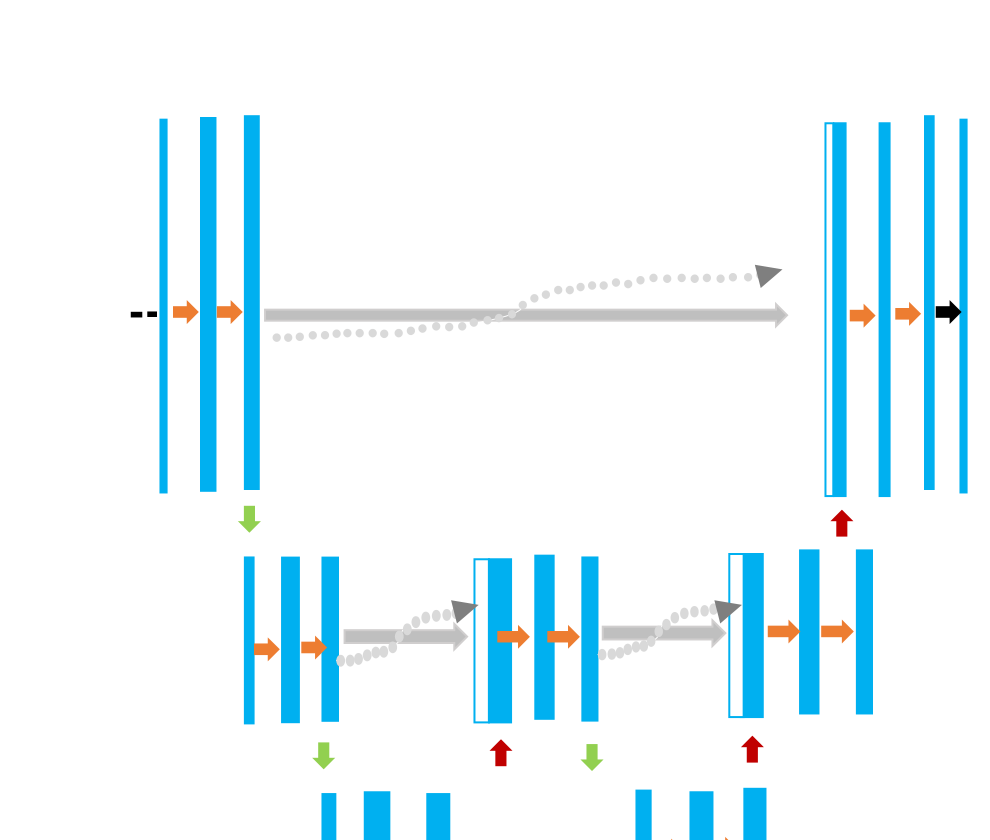
 The architectural layout of AIDUNet’s 2D and 3D versions is structured. All 2x 2 max pooling operations are applied to a layer with even x and y axes to enable the output segmentation map to be tiled continuously. Fundamental CNN elements such as currently downsampling convolutions, ReLUs, max-pooling, concatenations, sigmoid activation function, batch normalization, and dropouts are used in the architecture, which is similar to U-Net in this regard. But it’s important to emphasize the ensuing distinctive characteristics:

The CNN model is currently applicable to various image sizes due to a cropping process.

A classification layer that has been modified with a generalized dice loss function to accommodate different sorts of input data and image characteristics.

Significantly fewer learnable parameters and lower computational complexity than a U-Net with the same number of layers

In AID-U-Net, a number of contracting and expansive channels have been established. One main contracting path with the potential for additional up sampling paths exists in a one-sample AID-U-Net, as does one main up sampling path followed by the same number of sub-contracting paths.

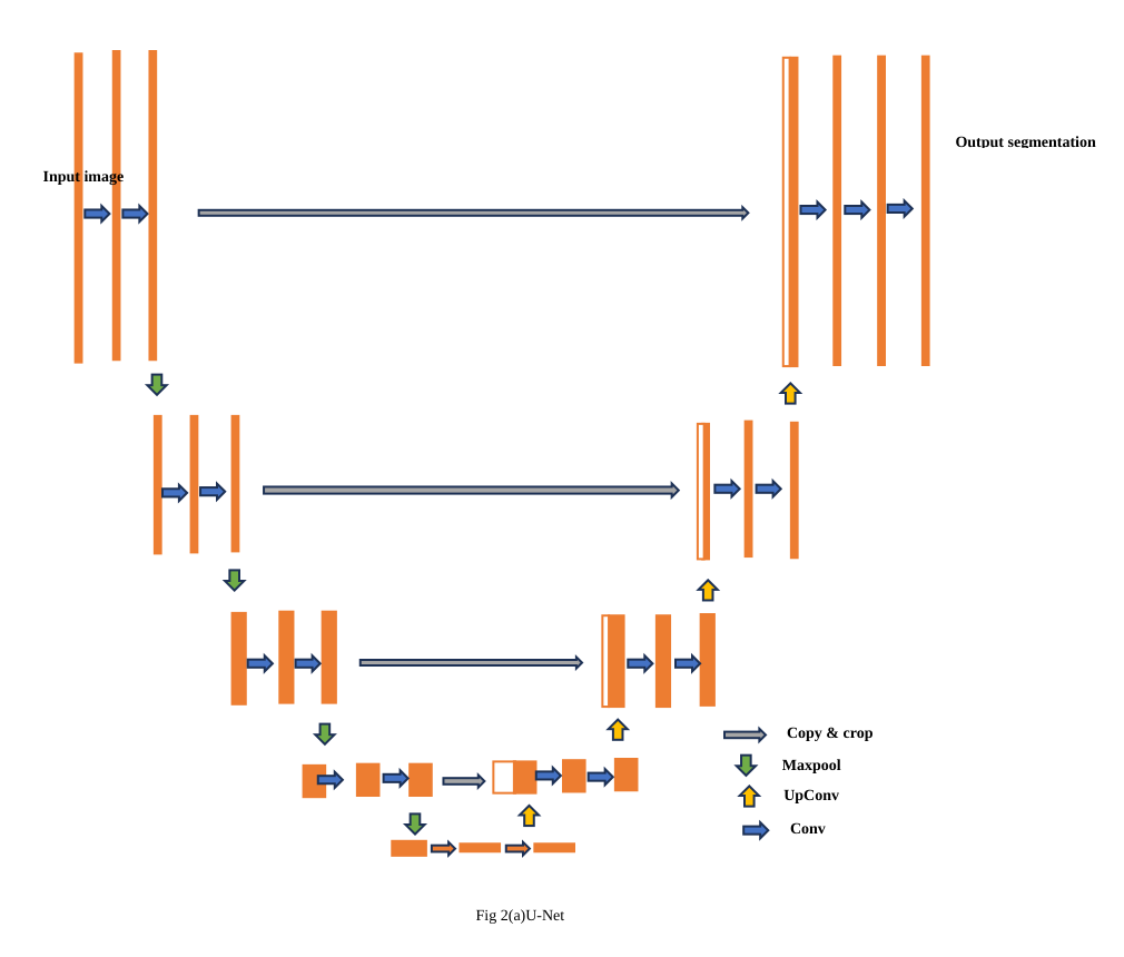
Output segmentation
Conv
UpConv
Maxpool
Copy & crop
Input image
Fig 2(a)U-Net

Conv
UpConv
Maxpool
Copy & crop
Fig :2(b)Proposed AID U-Net

Deep Layers Combinations and Block Formation in AID-U-Net

The foundation of AID-U-Net comprises two core trajectories: Contracting, downsizing input to matrices, and Expansive, fusing components for semantic segmentation output. Each route features distinct compositions:

Contracting: Successive convolution, Batch normalization, ReLU, convolution, Batch normalization, ReLU, dropout, and cropping layers constitute contracting blocks.

Expansive: Consecutive concatenation, Batch normalization, ReLU, convolution, Batch normalization, ReLU, and dropout layers compose expansive blocks.

For coherent block shapes, convolutions employ padding. The interlinking of contracting blocks involves max-pooling to curtail dimensions and pick crucial features.

Functionality of Downsampling (Contracting) and Upsampling (Expansive) Blocks

Linking consecutive expansive blocks, an up-convolutional layer facilitates upsampling of local features, channeling outcomes to output blocks. Concatenation layers within expansive blocks balance local and global features from the same rows. Instead of adding, concatenation preserves output variance by combining content from two layers in the expansive path. This ensures that the variance of each block’s output remains consistent with input layers. As a result, the network maintains the integrity of captured information during the expansion process, vital for effective semantic segmentation.

σ_output²=σ_{input1∥input2}²=σ_inputx² (10)

Here, X signifies the index of each input content to the concatenation layer ∥Unlike concatenation, an addition layer’s output would exhibit double the variance of each input assigned to that layer.

AID-U-Net’s output consists of two distinct layers:

The initial layer, a SoftMax layer, functions as an average pooling layer, harmonizing global features to create the ultimate semantic segmentation result. Following this is a consecutive layer with a sigmoid activation function, which serves as the classification layer, delivering the final outcome.

In every contracting block, a recurring process involves applying two convolutions (typically N filters with a 3×3 size and consistent padding). The first convolution is consistently succeeded by a batch normalization layer. This layer plays a pivotal role in orchestrating the outputs of convolutional layers, particularly during the feedforward phase. Its optimization occurs in a reverse learning phase. Batch normalization ensures the normalization of input variable activation, crucially within deployed mini-batches. This normalization framework facilitates elevated learning rates, contributing to efficient learning processes. The standardised output Y_I for each mini-batch is determined using the parameters and β and is calculated as follows:

Y_I=BN_γ,β(X_I)=γX_Î+β (11)

Both and β are dynamically updated during the backpropagation training iterations.

The selection between two classification layer loss functions—cross-entropy and dice coefficient—was evaluated, favoring the latter. This decision was influenced by the class imbalance within biomedical images, where certain segments encompass fewer pixels/voxels compared to others. The generalized dice loss function, denoted as L, quantifies the loss between predicted P and corresponding ground truth G:

l=1-(2∑_I=1^m(w_I∑_J=1ⁿ(p_IJg_IJ)))/(∑_I=1^m(w_I∑_J=1ⁿ((p_IJ²+g_IJ²)))) (12)

Here, m represents the number of classes, and n signifies the number of elements along the first two dimensions of p. The parameter w_I corresponds to the class contribution control weights. These weights are derived from the reciprocal of the anticipated region’s area for target objects. Their calculation follows this pattern:

w_I=(1)/((∑_J=1ⁿ(g_IJ))²) (13)

Each block also has layers for cropping, dropout, and batch normalisation in addition to the architectural sub-contracting and sub-expansive blocks.

Feature Extraction

To leverage highly informative features from segmented chromosome images, we employ transfer learning with pre-trained transformer models like Vision Transformer (ViT). These transformers automatically capture intricate patterns and dependencies, greatly enhancing chromosome structure detection accuracy. In addition to deep learning-based feature extraction, we integrate shape, color, and texture-based features to further improve the detection process. Geometric shape descriptors, color histograms, and texture descriptors like the proposed Improved Local Binary Patterns (LBP) complement the deep learning features, enabling precise characterization of chromosome structures. This multi-modal approach enhances the overall performance and reliability of chromosome analysis in medical imaging.

Vision Transformer

Transformers initially gained prominence in NLP tasks, exemplified by groundbreaking models like BERT and GPT-3. In contrast, the standard image processing approach relies on Convolutional Neural Networks (CNNs) with well-known architectures such as Xception, ResNet, EfficientNet, DenseNet, and Inception.

Transformers utilize attention to measure relationships between pairs of input tokens, such as words in a text. However, for images, computing relationships between all pixel pairs is computationally prohibitive. Vision Transformer (ViT) addresses this by computing relationships among pixels in smaller sections of the image, significantly reducing computational overhead. These sections, represented with positional embeddings, form a sequence fed into the Transformer. Each section’s embeddings, as learnable vectors, are transformed by an embedding matrix before being input to the Transformer along with the positional embeddings.

Similar to BERT, a crucial role in classification tasks is played by the class token. This special token serves as the sole input to the final MLP Head, having been influenced by all other tokens.

In image classification, the most common application, the Transformer Encoder is used to transform input tokens representing image sections. However, there are other applications where the decoder part of the traditional Transformer architecture is also employed, enabling tasks like image generation or image-to-image translation. This flexibility highlights the versatility of Transformers in diverse image-processing tasks beyond classification.

Texture Feature

Texture analysis involves assessing regions in an image based on their texture content. It aims to quantify perceptual qualities like roughness, smoothness, silkiness, or bumpiness by analyzing spatial variations in pixel intensities. By examining the patterns and structures present in an image, texture analysis provides valuable insights into the composition and nature of different regions. This process plays a crucial role in various image processing tasks, such as pattern recognition, segmentation, and classification, enabling more comprehensive and meaningful interpretations of visual data.

Local Binary Pattern

Local binary patterns between relations between neighbours: nLB

nLBP_D is established based on the connection between its neighbours around each pixel. The decimal equivalent of the binary series is determined by taking the 8 neighbours Q = Q₀, Q₁, Q₂,Q₃, Q₄,Q₅,Q₆, and Q₇ around the center pixel (P_c). Through comparisons, it is determined if a pixel is “1” or “0” depending on whether it is larger than the pixel after it. The example below demonstrates nLBP_D in operation. The nLBP_D method’s D variable indicates the distance. The distance between adjacent neighbours is specified by this parameter for comparison. For various values of the D parameter, different patterns are generated. A sample of how nLBP_D produces a binary pattern from various distances is illustrated in Fig. 2.

Fig. 2(a) illustrates a comparison of original sub-image and neighbour pixels in nLBP_D method, consequently, when the distance (D) is 1 (b), 2 (c), 3 (d).

To determined how the nLBP_D approach works the (P) pixels that are chosen around the center pixels are essential. The center pixel (P_c) and its neighbours Q = Q₀, Q₁, Q₂,Q₃, Q₄,Q₅,Q₆,Q₇ are included in the example below for D=1, D=2, D=3.

U= (P_c,Q₀, Q₁, Q₂,Q₃, Q₄,Q₅,Q₆,Q₇)

P_c=T(Q₀> Q₁),T(Q₁> Q₂ ), T(Q₂>Q₃ ), T( Q₃> Q₄), T(Q₄>Q₅), T(Q₅>Q₆ ), T(Q₆>Q₇), T(Q₇>Q₀) (14)

T(Q_j> Q_k)={1, &Q_j>Q_k, ; 0, &Q_j≥Q_k (15)

As shown in equation (15), when Q_j>Q_k, the binary equivalent value is “1”, otherwise the value is taken as an “0”.

For D = 1 the calculation of nLBP_D is shown in below (fig. 1(b)).

P_c=32>12|12>62|62>21|21>72|72>41|41>18|18>36|36>32

P_c=1, 0, 1, 0, 1, 1, 0, 1

P_c=(10101101)₂=(173)₁₀

Calculation of nLBP_D for D = 2 (fig. 1(c)).

P_c =T(Q₀> Q₂),T(Q₁> Q₃ ), T(Q₂>Q₄ ), T( Q₃> Q₅), T(Q₄>Q₆), T(Q₅>Q₇ ), T(Q₆>Q₀), T(Q₇>Q₁)

P_c=32>62|12>21|62>72|21>41|72>18|41>36|18>32|36>12

P_c=0, 0, 0, 0, 1, 1, 0, 0

P_c=(00001100)₂=(12)₁₀ (16)

Calculation of nLBP_D for D = 3 (fig. 1(d)).

P_c =T(Q₀> Q₃),T(Q₁> Q₄ ), T(Q₂>Q₅ ), T( Q₃> Q₆), T(Q₄>Q₇), T(Q₅>Q₀ ), T(Q₆>Q₁), T(Q₇>Q₂)

P_c=32>21|12>72|62>41|21>18|72>36|41>32|18>12|36>62

P_c=1, 0, 1, 1, 1, 1, 1, 0

P_c=(10111110)₂=(190)₁₀ (17)

Q₁₁
Q₆
Q₄
Q₃
Q₅
Q₂ Distance (D) = 1 Distance (D) = 2 Distance (D) = 3

Q₀Q₇

(b) (c) (d)

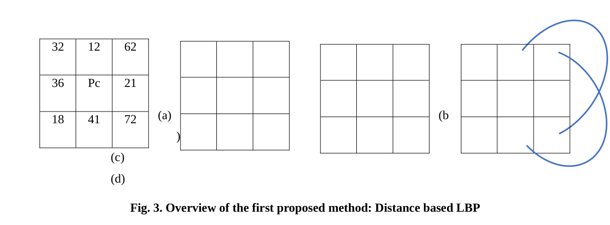
Fig. 3. Overview of the first proposed method: Distance based LBP

α=135^° α=90^° α=45^°

α=0^°

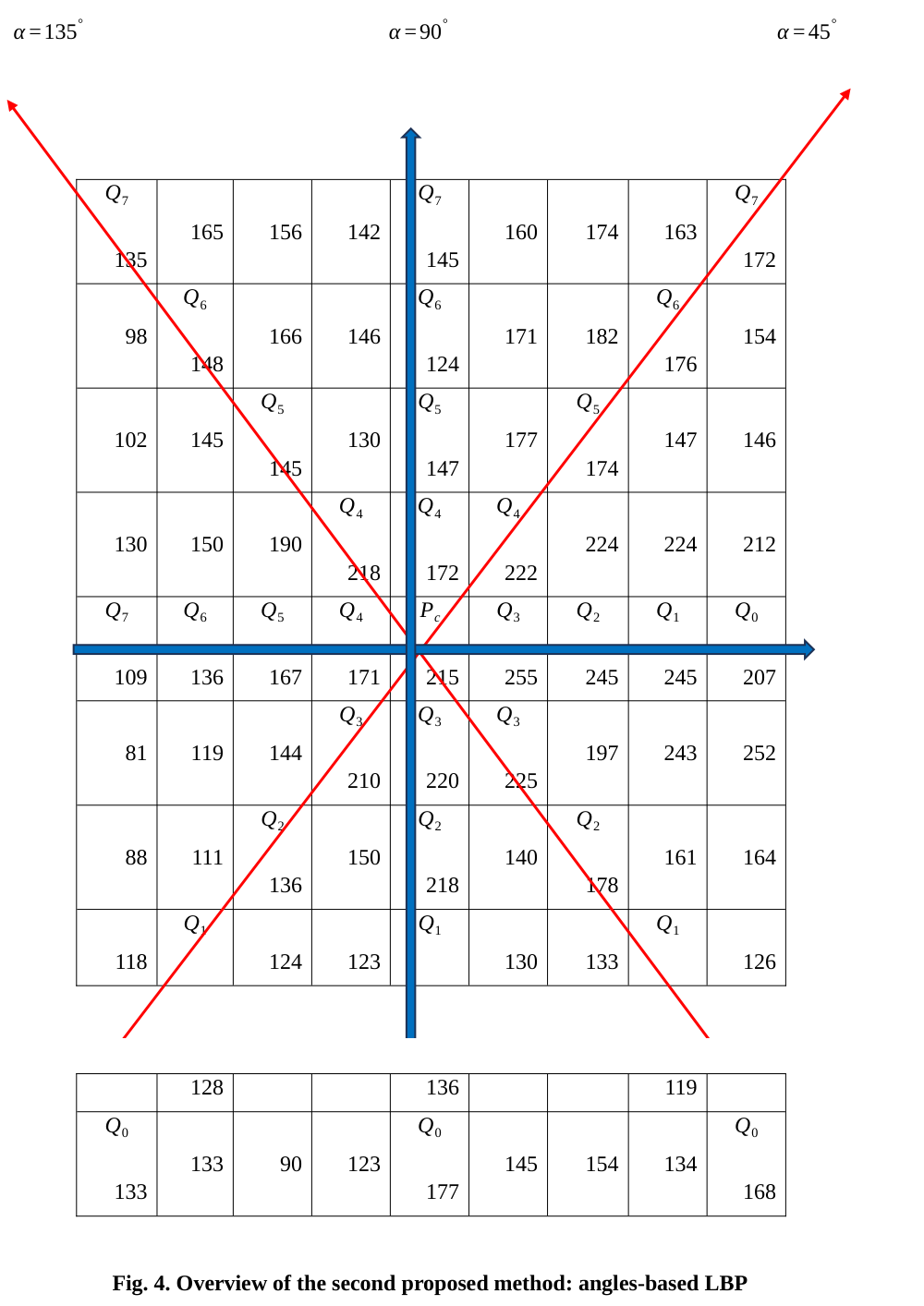
Fig. 4. Overview of the second proposed method: angles–based LBP

Numerous variations were obtained for different values of the D parameter, as can be observed from the examples that mentioned.

Local binary patterns based on angles: αLBP

LBP’s basic concept is relying on the notion that an image is composed of small patterns. The distribution of specific characteristics within a picture is outlined by the histogram of these micro patterns.

Based on an angle value, the αLBP operator determines the value of each pixel. The angles are calculated to have values of α= 0, 45, 90, and 135 degrees. According to the angle value, neighbours (Q = {Q₀, Q₁, Q₂,Q₃, Q₄,Q₅,Q₆,Q₇}) are assessed on the plane passing over the center pixel (P_c). When the center pixel is compared to its neighbours on the drawn plane, the value of P_c is labeled as 1 if P_c > P_j, and “0” in all other circumstances. After the labeling operation A 8-bit binary code is obtained, and this binary code is subsequently converted into a decimal number. The center pixel PC is represented by this decimal number. Eq. (18) is utilized to compute the LBP value. In the illustration below, an example of its computation process is presented.

αLBP=∑_j=0^Q((v(P_j-P_c))2^j (18)

The LBP operator is computed for two distinct horizontal and two different vertical angles, as illustrated in Fig. 4. LBP operators that were estimated using various angles diverged from one another.

It is expected that the strategy of looking for patterns at various angles will work well in a variety of textural issues. Below are LBP operators that were produced using the various angles depicted in Fig. 4.

Calculation of αLBP_D for α = 0;

P_c =T(Q₀> Q_c),T(Q₁> Q_c ), T(Q₂>Q_c ), T( Q₃> Q_c), T(Q₄>Q_c), T(Q₅>Q_c ), T(Q₆>Q_c), T(Q₇>Q_c)

P_c=T(207> 215),T(245> 215), T(245>215 ), T( 255> 215), T(171>215), T(167>215 ), T(136>215), T(109>215)

P_c=0, 0, 0, 0, 1, 1, 1, 0

P_c=(00001110)₂=(14)₁₀ (19)

Calculation of αLBP_D for α = 45;

P_c =T(Q₀> Q_c),T(Q₁> Q_c ), T(Q₂>Q_c ), T( Q₃> Q_c), T(Q₄>Q_c), T(Q₅>Q_c ), T(Q₆>Q_c), T(Q₇>Q_c)

P_c=T(133> 215),T(128> 215), T(136>215 ), T( 144> 215), T(222>215), T(174>215 ), T(176>215), T(172>215)

P_c=0, 0, 0, 0, 1, 0, 0, 0

P_c=(00010000)₂=(16)₁₀ (20)

Calculation of αLBP_D for α = 90;

P_c =T(Q₀> Q_c),T(Q₁> Q_c ), T(Q₂>Q_c ), T( Q₃> Q_c), T(Q₄>Q_c), T(Q₅>Q_c ), T(Q₆>Q_c), T(Q₇>Q_c)

P_c=T(177> 215),T(136> 215), T(218>215 ), T( 220> 215), T(172>215), T(147>215 ), T(124>215), T(145>215)

P_c=0, 0, 0, 0, 1, 1, 0, 0

P_c=(00001100)₂=(12)₁₀ (21)

Calculation of αLBP_D for α = 135;

P_c =T(Q₀> Q_c),T(Q₁> Q_c ), T(Q₂>Q_c ), T( Q₃> Q_c), T(Q₄>Q_c), T(Q₅>Q_c ), T(Q₆>Q_c), T(Q₇>Q_c)

P_c=T(168> 215),T(119> 215), T(178>215 ), T( 225> 215), T(218>215), T(145>215 ), T(148>215), T(135>215)

P_c=0, 0, 0, 1, 1, 0, 0, 0

P_c=(00011000)₂=(24)₁₀ (22)

Color Features

Intensity values used in color spaces serve as a representation of color. By employing the color space method, we can define, see, and produce colors. Global approaches and local methods are two main categories that describe how color features are extracted. Global approaches consider the entire image throughout the feature extraction process, including the global color histogram, the intersection of the histograms, the image bitmap, etc.

Color Histogram

The color histogram presents the image from various angles. A color histogram is used to express the frequency distribution of colors in an image, and it also counts and stores related pixels. The color histogram examines each statistical color frequency present in an image. The color histogram not only focuses on specific areas of a picture, but also solves problems with translation, rotation, and angle of view. The indexing and retrieval of image databases rely heavily on local color histograms since they are simple to calculate and robust to even the smallest alterations in the image.

Optimal Feature Selection

To optimize the feature space and reduce dimensionality, propose a novel hybrid optimization algorithm that combines the Dwarf mongoose optimization algorithm and the Prairie dog optimization algorithm. This advanced technique intelligently identifies the most relevant and discriminative features, ensuring the detection model focuses on the most informative aspects of chromosome structures.

Hybrid Optimization

Initialization

Initialization involves randomly assigning positions to the PDs within a multi-dimensional space. These PDs act as search agents, each representing a point in the space. In PDO, PDs are organized into coteries, and each PD belongs to a specific coterie, reflecting their collaborative nature. The matrix, denoted as CT, encodes the positions of these coteries within the colony, facilitating the group dynamics of the optimization process. This random initialization sets the starting point for the search in the algorithm.

ct=[[ct_1,1 , ct_1,2 , ⋯ , ct_1,D-1 , ct_1,D] ; [ct_2,1 , ct_2,2 , ⋯ , ct_2,D-1 , ct_2,D] ; [⋮ , ⋮ , ct_I,J , ⋮ , ⋮] ; [ct_m,1 , ct_m,2 , ⋯ , ct_M,D-1 , ct_M,D]] (23)

The equation (24) below defines the spatial coordinates of individual search agent within a specific coterie, denoted as ct_I,J, representing the ith coterie’s jth dimension.

pd=[[pd_1,1 , pd_1,2 , ⋯ , pd_1,D-1 , pd_1,D] ; [pd_2,1 , pd_2,2 , ⋯ , pd_2,D-1 , pd_2,D] ; [⋮ , ⋮ , pd_I,J , ⋮ , ⋮] ; [pd_N,1 , pd_N,2 , ⋯ , pd_N,D-1 , pd_N,D]] (24)

These equations utilize uniform distributions for the positioning of both CT and PD along their respective dimensions pd_I,J.

ct_I,J=u(0,1)*(ub_J-lb_J)+lb_J (25)

pd_I,J=u(0,1)*(UB_J-LB_J)+LB_J (26)

𝑈𝐵𝑗 and 𝐿𝐵𝑗 are determined by uniformly distributed random values 𝑈(0, 1), within the bounds 𝑢𝑏𝑗 and 𝑙𝑏𝑗 for the 𝑗th dimension.

Fitness computation

Calculate the fitness function value (𝑓) for each search agent position based on the problem-specific fitness function. The fitness function is a mapping from the position of a search agent (𝑃𝐷) to a scalar fitness value

fit=max((A)) (27)

Where A is th accuracy in Eq. (27)

f(pd)=[[f₁([pd_1,1 , pd_1,2 , ⋯ , pd_1,D-1 , pd_1,D])] ; [f₂([pd_2,1 , pd_2,2 , ⋯ , pd_2,D-1 , pd_2,D])] ; [⋮ , ⋮ , , ⋮ , ⋮] ; [f_N([pd_N,1 , pd_N,2 , ⋯ , pd_N,D-1 , pd_N,D])]] (28)

Alpha Group

After the population has been commenced, the effectiveness of each solution is evaluated. The likelihood value is calculated by Eq. (29) and the alpha female is selected using this likelihood.

∝=(fit_I)/(∑_I=1^N(fit_I)) (29)

The number of search agent in the ∝ is represented by the N-BR symbol. Where BR is the number of babysitters and peep is the vocalization made by the dominant female who keeps the family on track. The following describes how the solutions update method works.

x_I+1=x_I+PH_I*peep (30)

where PH_I is a randomly generated number. After each iteration, the sleeping mound is depicted in Eq. (30), where PH_Iis a uniformly distributed random integer between [1, 1].

RI_M=(fit_I+1-fit_I)/(max⁡[|fit_I+1-fit_I|]) (31)

Eq. (31) provides the average number of the discovered sleeping mounds.

φ=(∑_I=1^N(RI_M))/(N) (32)

When the childcare exchange need has been met, the algorithm moves on to the scouting phase, when the next food source or resting mound is taken into account.

Scout Group

If the family forages pretty far in the scout group section, they will come to observe a suitable sleeping mound. Eq. (33) simulates the scout search agent.

x_I+1={x_I-cf*PH_I*rand[x_I-m]⃗, if φ_I+1>φ_I ; x_I+cf*PH_I*rand[x_I-m]⃗, otherwise (33)

where rand is a random number between [0, 1], cf and m⃗ values are determined by Eq. (34) and (35), respectively.

cf=(1-(iter)/(Max_iter))^{(2*(iter)/(Max_iter))} (34)

m⃗=∑_I=1^N((x_I*rM_I)/(x_I)) (35)

Babysitters are often lower-class group members who stay with the kids and rotate their places frequently so the alpha female (mother) can lead the rest of the squad on daily hunting expeditions

In this optimization scenario, the top-performing solution, often referred to as the Alpha Group, stands as the premier choice. Following closely behind, solutions ranked from 2nd to 5th collectively constitute the Scout Group, responsible for exploring and expanding the search space. Meanwhile, solutions ranked 6th to 10th are known as the Babysitters, tasked with overseeing and nurturing less competitive solutions, ensuring the overall optimization process runs smoothly. This hierarchical arrangement enables efficient and effective optimization strategies.

Exploration

In this section, the PDO exploratory approach, this method involves utilizing the foraging and burrow-building behaviors of the PDs to explore the optimization problem domain. PDs construct intricate tunnels centered around abundant food sources. When their current food source depletes, they embark on extensive searches across the colony or problem space to locate new sustenance or solutions. They then establish fresh tunnels around each newfound resource. These burrows serve dual purposes, providing both environmental stability and protection against predators. PDs reside in organized colonies, divided into family units or coteries, each with its own territorial borders. The presence of a predator is the sole factor that compels these coteries to temporarily halt their communal activities of feeding and burrow excavation within their defined territories.

PDO determines its exploration and exploitation phases based on four criteria, dividing the maximum iterations into two exploration and two exploitation parts. The two exploration techniques are interconnected, relying on each other for the PDO optimization process to effectively navigate the search space.

(i)iter < Maxiter/4

pd_I+1,J+1=gbest_I,J-ecbest_I,J×ρ-cpd_I,J×Brownian(n)∀iter<(Max_iter)/(4) (36)

During the exploration phase, coterie members initially spread out to locate fresh food sources. Their motion, resembling Brownian motion, involves occasional large hops, preventing exhaustive searches in one area but effectively covering diverse regions for exploration. They communicate discoveries through distinctive noises. Based on food quality, the best source is selected for foraging, and new burrows are constructed. Equations below govern foraging position updates in this algorithmic exploration phase.

(ii) (Max_iter)/(4)≤Iter<(Max_iter)/(2)

pd_I+1,J+1=gbest_I,J×Rpd×ds×Brownian(n)∀(Max_iter)/(4)≤Iter<(Max_iter)/(2) (37)

In this context, ecbest_I,J represents the evaluation of the impact of the most superior solution obtained globally, while gbest_I,J signifies the best solution available worldwide. Rpd denotes the position of a randomly chosen solution, and cpd_I,J represents the cumulative effect resulting from all search agents within the colony. Additionally, ρ represents the specialized food source alarm frequency set at 0.1 kHz for the experiment’s specific context. These variables play essential roles in the PDO algorithm’s operation.

(iii) 𝑖𝑡𝑒𝑟 ≥ 𝑀𝑎𝑥𝑖𝑡𝑒𝑟/2

pd_I+1=α+π*rand*(pd_I-pd_K) (38)

In this context, the term π=((peep)/(2))*rand*ω, x_I represents the previous position of a search agent, while rand is a randomly generated number within the range [-1, 1]. pd_K refers to a randomly chosen search agent within the optimization process.

Exploitation

This section provides a comprehensive overview of PDO’s exploitation strategies, PDO capitalizes on the differential responses of PDs (search agent) to two distinct communication signals or alarms. These signals can convey various information, from predator presence to available food sources. PDs’ exceptional communication skills facilitate meeting their nutritional needs and defending against predators. They can also share insights about food quality and predator behavior. PDs respond differently to these signals; for instance, reliable food signals lead them to gather for feeding, while hawk alerts prompt some to hide while others keep watch. These behaviors encourage PDs to converge, simulating a promising location for further exploration (exploitation) in PDO. Exploitation strategies are designed to thoroughly investigate potential regions identified during the exploration phase. The equation below outlines the two tactics employed in this phase, with PDO switching between them based on specific conditions.

(1)/(2) Max_iter ≤ iter ≤ 3/4 Max_iter

pd_I+1,J+1=gbest_I,J-ecbest_I,J×ε-cpd_I,J×rand∀(Max_iter)/(2)≤Iter<(3)/(4)Max_iter (39)

In this context, ecbest_I,Jassesses the influence of the most recently acquired top-quality solution, while gbest_I,J represents the best global solution attained thus far. The variables 𝑖𝑡𝑒𝑟 and Max_iter denote the current iteration and the maximum allowable iterations, respectively. 𝜀 signifies a small value indicating food quality, and cpd_I,J represents the collective impact of all PDs within the colony

(ii) 3/4 Max_iter < 𝑖𝑡𝑒𝑟 ≤ Max_iter

pd_I+1,J+1=gbest_I,J×pe×rand ∀(3)/(4)Max_iter<Iter≤Max_iter (40)

. Furthermore, rand is a random number drawn from the range 0 to 1, contributing to the stochastic nature of PDO’s exploitation phase and the predator effect is pe.

(iii) iter < 1/2 Max_iter or iter > Max_iter

x_I+1=(x_J+rand*(α-(x_K+x_H)/(2)*BR) (41)

In the PDO algorithm, the process of replacing the babysitters with search agent is governed by random selection. The selected search agent, denoted as x_J, x_K, and x_H, serve as new search agents and convey their information to the babysitters. Additionally, the variable BR represents the birthrate, which influences the frequency of such agent replacements.

Scout for New Food Sources

Allow search agent designated as scouts to search for new food sources or optimal solutions based on the leader’s communication. Update scout positions accordingly. The scout’s position update equation may resemble that of leaders but with variations to adapt to scouting behavior.

l={Roundup(0.6*n*dim*((1)/(c_Iter))) ; l* c_Iter*cf when l<0 , (42)

When l reaches zero, it undergoes a reset operation by multiplying it with the current iteration number and CF.

Communicate and Exchange Information

Enable communication between search agnet to share information about food sources, threats, and promising locations. Implement information exchange mechanisms, such as the exchange of positions or specific signals, among search agent as in IDMO. The details of communication and exchange mechanisms would depend on the algorithm design. Each search agent can send signals to nearby search agent within a certain radius R. A search agent signal strength decreases with distance. Here’s a simplified expression for communication:

Signal Strength (S) from Search agnet I to Search agent J:

s_IJ=((1)/(Euc_IJ)), if Euc_IJ≤r (43)

s_IJ=0, if Euc_IJ>r (44)

Update Positions of Search agent

Update positions of all search agent based on their roles (leaders, scouts, regular Search agent) using appropriate position update equations for exploration and exploitation phases. The specific position update equations may vary for each group based on their roles and behaviors.

The position update equations can vary based on the roles (leaders, scouts, regular search agent). Below are simplified examples:

For Regular search agent:

pd_I+1,J+1=pd_I,J+α*(gbest_I,J-pd_I,J)+β*rand⃗ (45)

For Scouts (Exploration):

pd_I+1,J+1=random position within search space

For Leaders (Exploitation)

pd_I+1,J+1=pd_I,J+γ*(gbest_I,J-pd_I,J)+δ*rand⃗ (46)

Here, α, β, γ, and δ are weight factors to control the influence of various factors.
rand⃗ represents a random direction within the search space, and bestPosition is the best position found so far by the individual or group.

Termination Criteria

Save the so far acquired global best gbest_I,J and position best solution pd.

Return the gbest_I,J and pd.

Chromosome Structure Detection

To enhance the robustness of chromosome structure classification, introduce Chromo Ensemble Net, an innovative architecture that capitalizes on the strengths of several classifiers like DenseNet, ResNet, Efficient Net, and Random Forest. By leveraging a voting approach, the Chromo Ensemble Net combines the predictive abilities of these diverse classifiers. This ensemble approach allows efficient feature reuse and gradient flow, leading to more precise and reliable chromosome structure detection. By harnessing the collective intelligence of multiple classifiers, Chromo Ensemble Net improves the accuracy and robustness of the classification task.

ChromoEnsemble Net

DenseNet

Densely Connected Convolutional Networks (DenseNet) represents a pivotal architecture in the realm of convolutional neural networks (CNNs). Unlike traditional CNNs, DenseNet employs a unique approach by connecting each layer to every other layer within the network. This innovation promotes more efficient learning by fostering feature reuse and reducing parameter count while improving gradient flow during training. The core idea behind DenseNet is elegantly simple: by concatenating feature maps from all preceding layers, every layer gains access to the collective knowledge of its predecessors. This stands in contrast to conventional CNNs, where each layer only taps into the immediate preceding layer’s features. DenseNet comprises dense blocks and transition layers, with each layer in a dense block connected to every other layer, forming “shortcut” links. Transition layers work to downsize feature maps between dense blocks, facilitating network growth. DenseNet excels in various computer vision tasks, including image classification, object recognition, and semantic segmentation, consistently achieving state-of-the-art performance thanks to its efficient feature reuse and parameter reduction mechanisms.

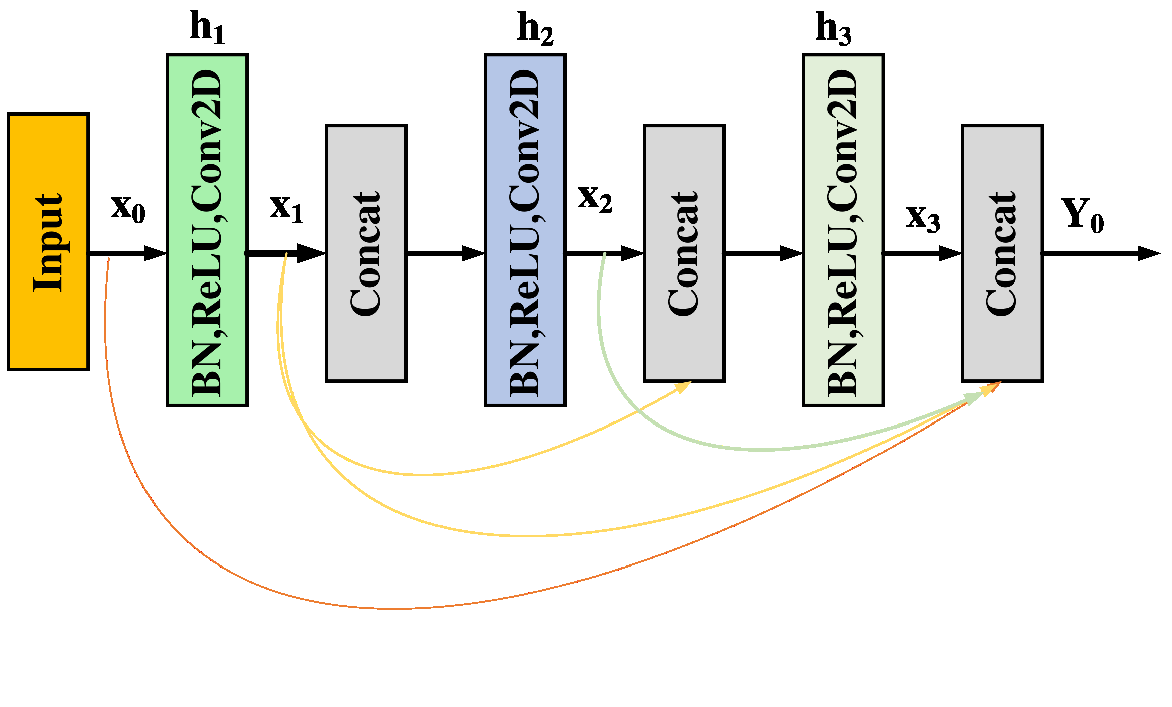
Figure 5: Architecture of DenseNet

ResNet

Residual Neural Network (ResNet) achieved a groundbreaking ImageNet Large Scale Visual Recognition Challenge (ILSVRC). ResNet’s defining innovation lies in its incorporation of residual connections between network layers, a design feature that substantially reduces training loss, safeguards knowledge transfer, and significantly enhances overall performance. The essence of a residual connection is that a layer’s output is formed by convoluting its input and adding the input itself, creating a “shortcut” for information flow. A visual representation of the ResNet model’s architecture is depicted in Figure 6, highlighting the unique and impactful design principles that underpin its success in the realm of deep learning and computer vision.

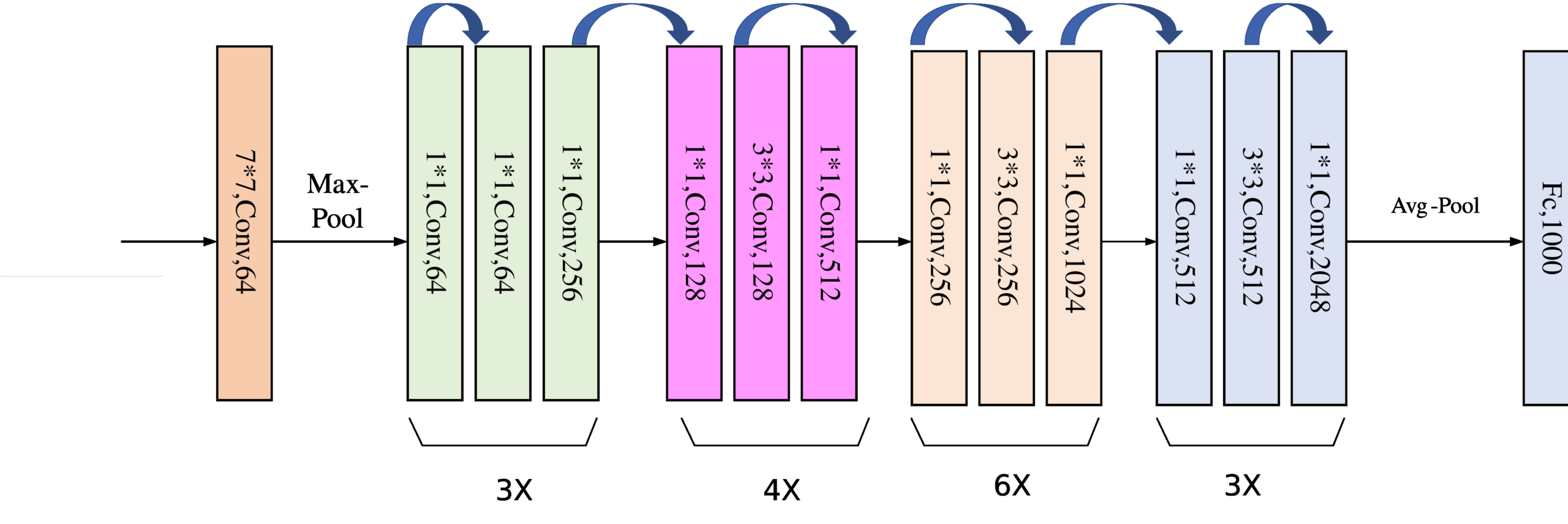
Figure 6 :Architecture of ReNet 50

EffcientNet

EfficientNet of convolutional neural networks (CNNs). It introduces a groundbreaking approach to effectively scale and design CNNs, meticulously considering critical factors like depth, width, and resolution. By leveraging compound coefficients, EfficientNet strikes a harmonious balance among these dimensions, resulting in heightened model performance. What truly distinguishes EfficientNet is its ability to amplify network capabilities while maintaining architectural integrity. This achievement is realized through a systematic coefficient determination process involving grid search techniques, ensuring the optimal configuration of network elements. Furthermore, EfficientNet adheres to predefined constraints, trimming unnecessary parameters, ultimately yielding more efficient and potent CNNs with diverse applications across computer vision and deep learning domains.

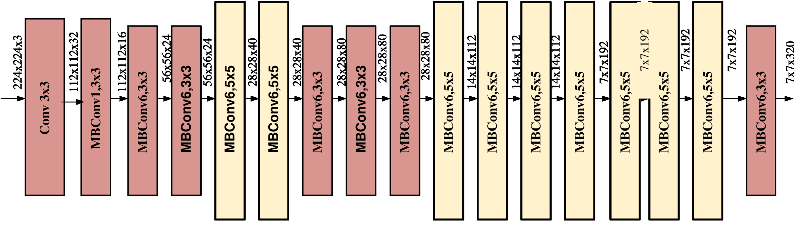
Figure 7: Basic architecture of EfficientNet

The architectural innovation of EfficientNet introduces a distinctive inverted structure through the pioneering Mobile Inverted Convolution (MBConv) method, notably known as the Inverted Residual Block. This design incorporates sum-product operations and integrates skip connections within compact segments, efficiently reducing channel dimensions while preserving the initial channel count. MBConv’s narrow-wide-narrow approach diverges from conventional Convolutional networks. It achieves parameter reduction through a 3×3 Depth-wise Convolution, widens channels with a 1×1 Convolution, and then further compresses channels via another 1×1 Convolution. Remarkably, the EfficientNet-B7 model excels by scaling dimensions while maintaining high accuracy for each parameter, yielding a compact yet remarkably precise architectural solution in the landscape of deep learning.

Random Forest

The Random Forest algorithm, a popular supervised machine learning technique, stands out for its widespread use, accuracy, simplicity, and versatility. It boasts applicability in both classification and regression tasks, owing to its inherent nonlinearity, rendering it highly adaptable across various datasets and scenarios. The name “forest” reflects its core principle of growing a multitude of decision trees, with their collective wisdom used to make more precise predictions. Unlike a solitary decision tree, which offers limited outcomes, the forest delivers heightened accuracy by considering a broader spectrum of groups and decisions. Furthermore, it injects an element of randomness into the model by selecting the optimal feature from a randomized subset, enhancing its robustness and predictive power

Detected Outcome

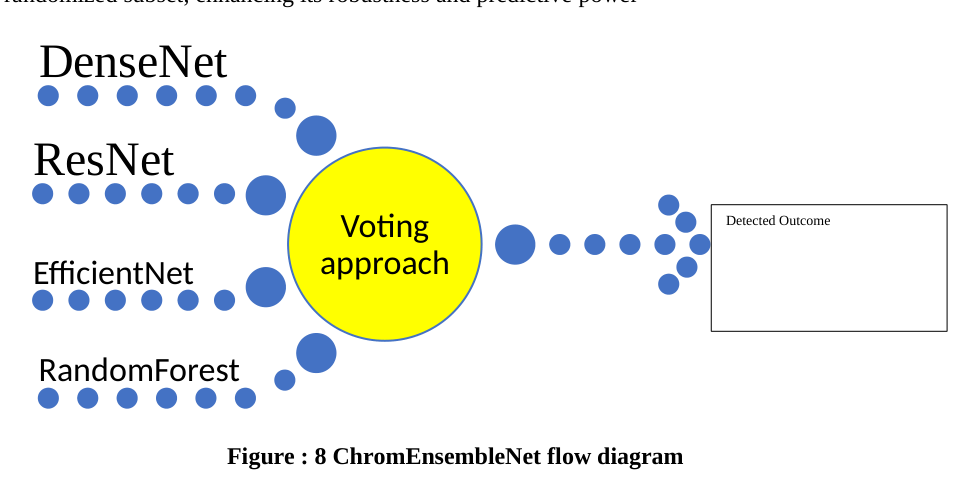
Figure : 8 ChromEnsembleNet flow diagram

ChromoEnsembleNet is the solution for robust chromosome structure classification. It harnesses the collective strengths of several classifiers, such as DenseNet, ResNet, EfficientNet, and Random Forest, utilizing a voting approach. This innovative architecture promotes effective feature reuse and gradient flow, culminating in highly accurate chromosome structure detection. By amalgamating the predictive capabilities of these diverse classifiers, ChromoEnsembleNet achieves exceptional precision, ensuring its efficacy in medical image analysis for the identification of chromosomal abnormalities and genetic disorder diagnosis.

Result And Discussion

Training accuracy and testing accuracy must be distinguished: Table 2 reports 0.998 and 0.961 respectively. The listed testing counts, if interpreted as TP 264, TN 257, FP 10 and FN 13, imply 521 correct predictions in 544 cases, or approximately 95.77%, rather than 96.1%. The count labels and several rates are inconsistent, and the averaging procedure and evaluation population are insufficiently specified. The numerical table and original plots are retained as reported, without treating them as independently verified diagnostic performance.

Experimental Setup

In this research , to get the best accuracy in the proposed model, the model is trained and tested in PYTHON and Carrier type dataset with the performance metrics Accuracy, Precision, Recall, F1-Score, Sensitivity, FPR, Specificity, FNR, TNR, and TPR. The proposed model is trained and tested using Python, and performance metrics include accuracy, TNR, specificity, sensitivity, precision, F1-score, recall, TPR, FNR, and FPR, as shown in Table 2. Table 2 reports training accuracy of 0.998 and testing accuracy of 0.961 and training and testing precision of 0.996 and 0.974, respectively. Additionally, while training the proposed model, its recall value is 1, its sensitivity is 0.932, its F1-Score is 0.998, its specificity is 0.902, its TNR is 531, its FPR is 1, and its FNR is 0. Recall is 0.95, sensitivity is 0.932, F1-Score is 0.962, specificity is 0.902, TNR is 257, FPR is 10, TPR is 264, and lastly, FNR is 13. These values are obtained when testing the suggested model. By using the hybrid optimisation approach, it is clear that the proposed model has the best accuracy.

Table 2: Overall Performance metrics of the proposed model

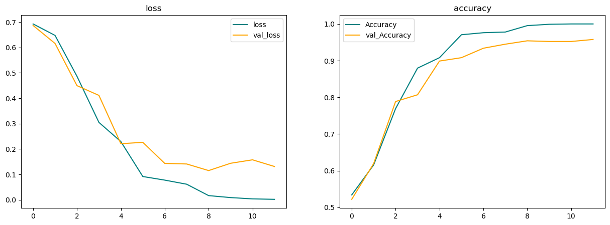
Figure 9: Graphical format of loss and accuracy of the proposed model

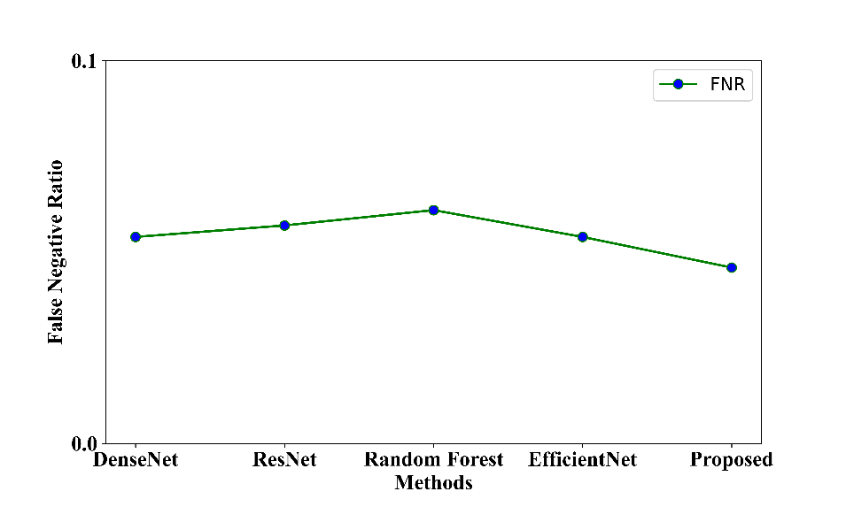
Figure 10: Graphical representation of the FNR of the proposed model

Fig 10 illustrates the graphical format of the False negative ratio of the proposed model with the other comparable models.From this it is clear that the False negative Ratio of the proposed model is very low when it is compared with the models like DenseNet, ResNet, Random forest methods, EfficientNet False negative Ratio.

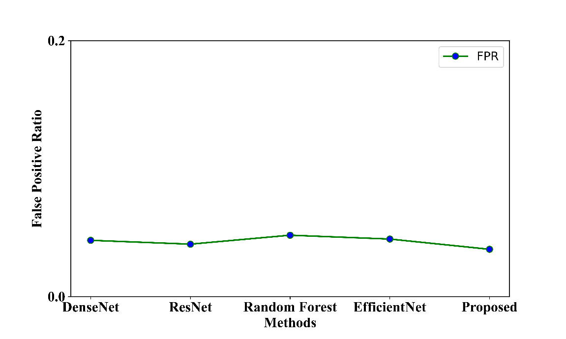
Figure 11: Graphical representation of the False Positive Ratio of the proposed model

Fig 11 illustrates the graphical format of the False positive ratio of the proposed model with the other comparable models.From this it is clear that the False negative Ratio of the proposed model is lower than the other comparable models like DenseNet, ResNet, Random forest methods, EfficientNet False positive Ratio.

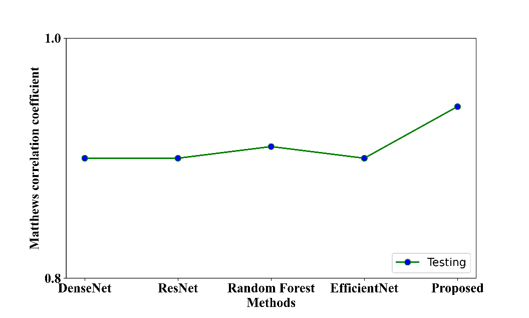
Figure 12: Graphical representation of the MCC of the proposed model

Fig 12 illustrates the graphical format of the MCC of the proposed model with the other comparable models. From this it is clear that while on testing the MCC value of the proposed model is very high when it is compared with the models like DenseNet, ResNet, Random forest methods, EfficientNet MCC value.

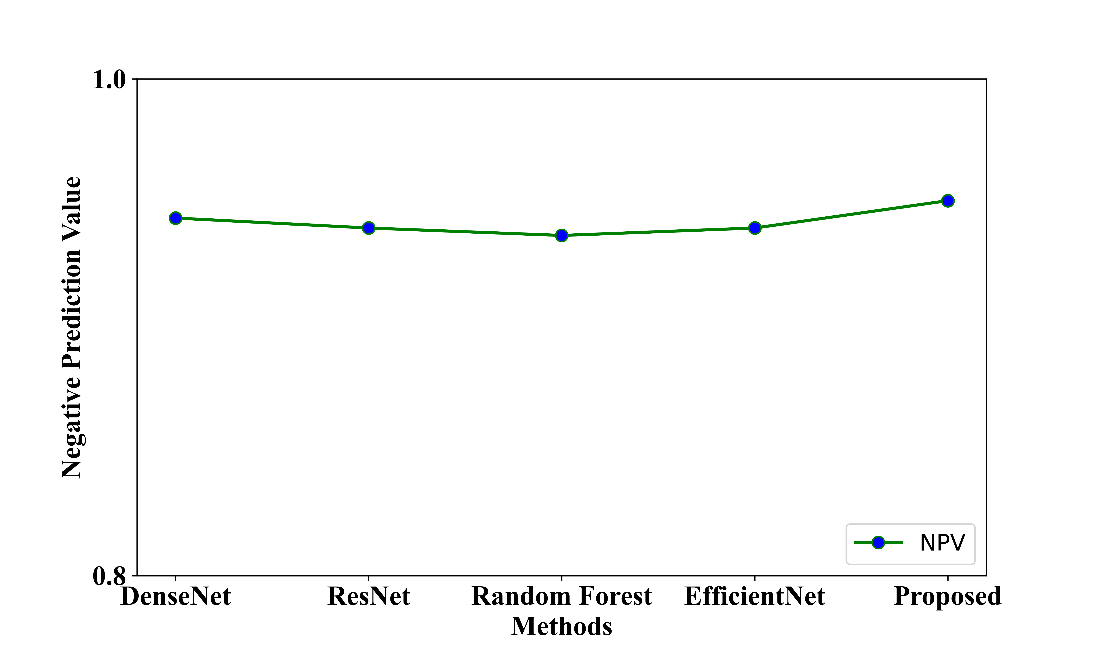
Figure 13: Graphical representation of the NPV of proposed model

Fig 13. Represents the graphical representation of the Negative prediction Value of the proposed model with the other comparable models. The Negative Prediction value of the proposed model is high rather than the comparable models like DenseNet, ResNet, Random Forest Method and EfficientNet Negative Prediction Value.

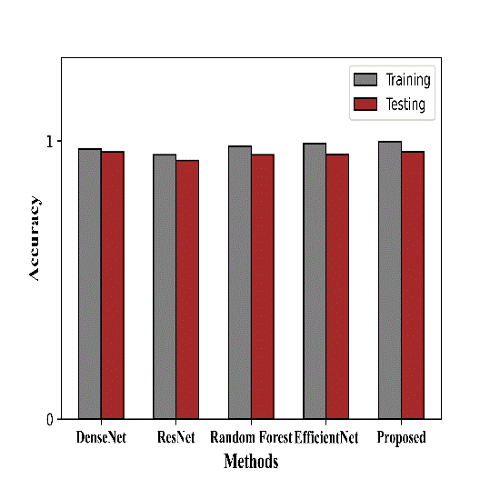
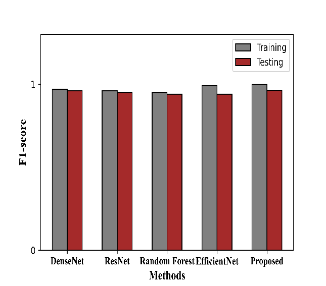
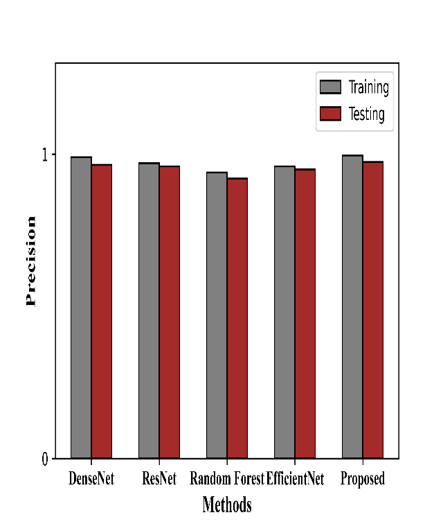
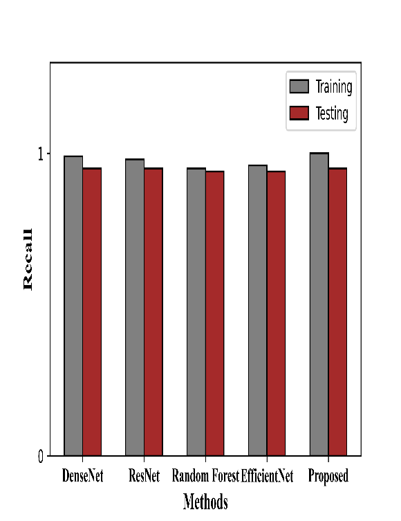
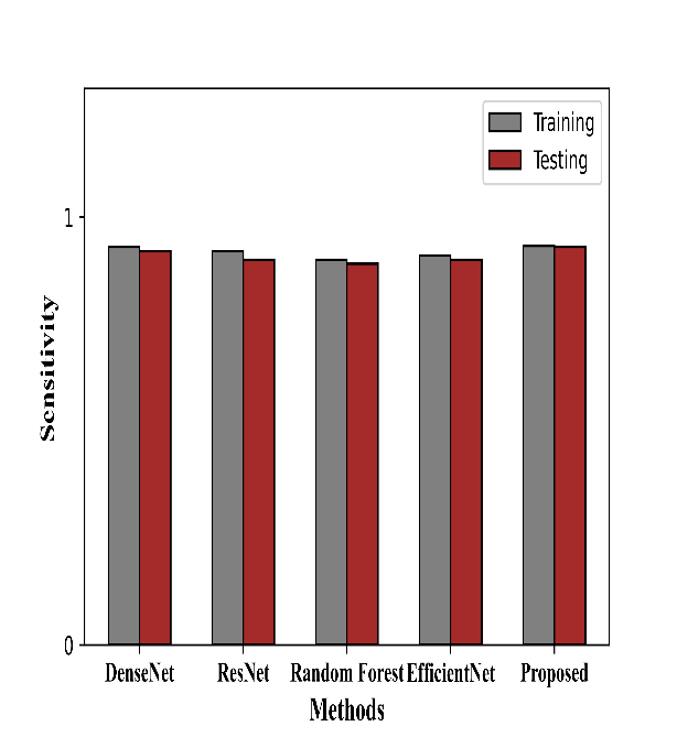
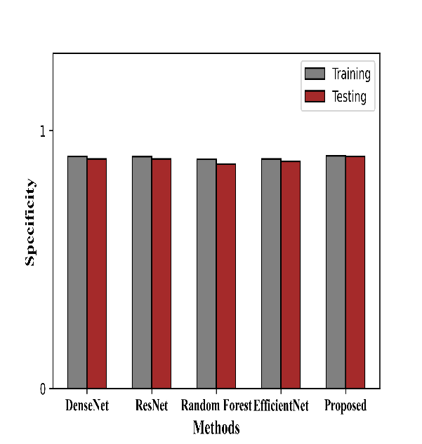
Figure 14: Graphical format of the Performance metrics (a ) accuracy (b) F1-Score (c ) Precision (d) Recall (e ) Sensitivity (f ) Specificity of the proposed model

Fig 14 illustrates the graphical Format of the performance metrics like accuracy , F1-Score, Precision, Recall, Sensitivity, Specificity of the proposed model with the other models. While on Testing and Training the proposed models accuracy , Precision, F1-Score, Recall, Sensitivity, Specificity is high than the other models like DenseNet, ResNet, Random Forest methods, Efficient Net. These are all due to the optimization process.

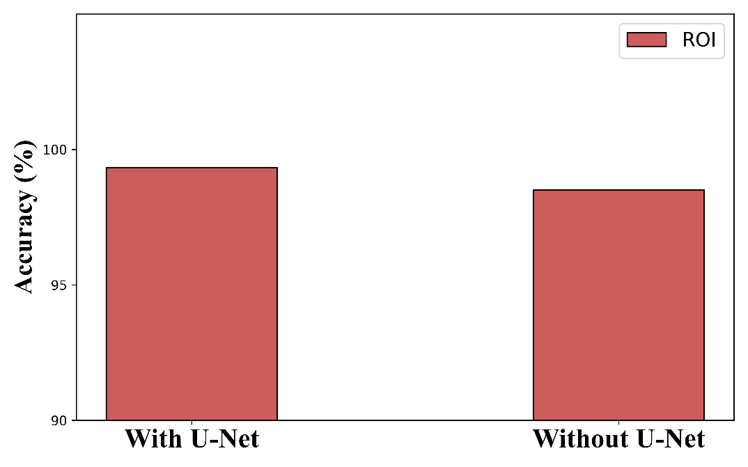
Figure 15: Graphical format of Segment With and Without U-Net

Segment with and Without U-Net of the proposed model accuracy is illustrated in Fig. 15. By Segment with U-Net the proposed model Region Of Interest accuracy is high and at the same time the segment without U-Net the proposed model Region Of Interest accuarcy is low.

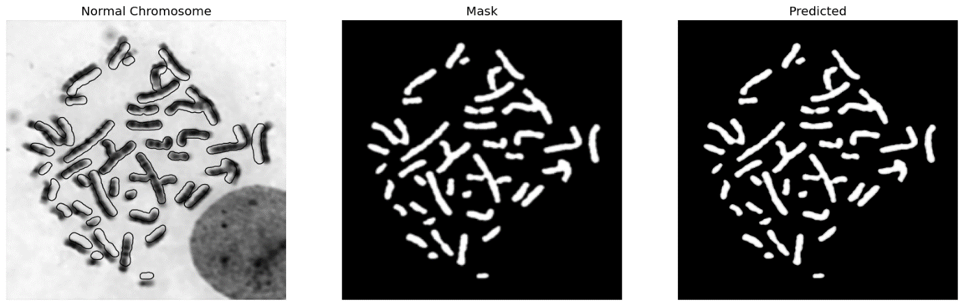
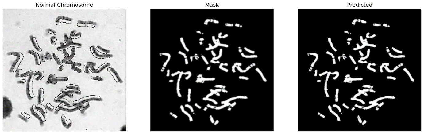
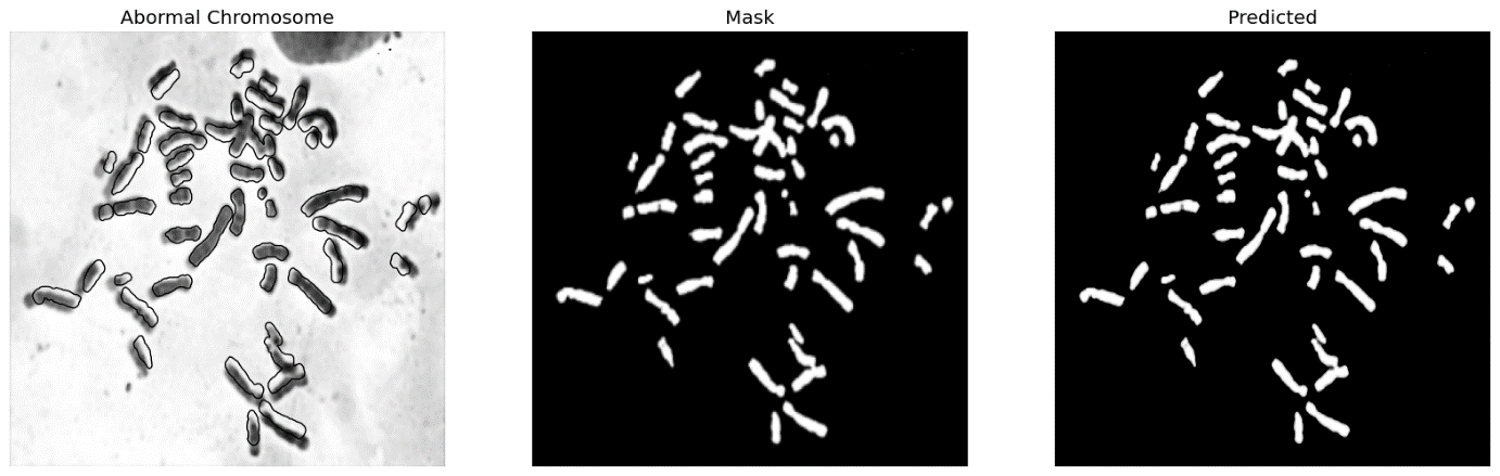
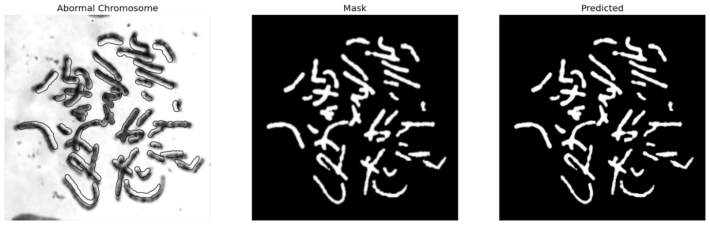
Figure 16 : Sample Normal and abnormal images of chromosome; (a ) and (b) Normal chromosome , mask and predicted images; (c) and (d) Abnormal chromosome, mask and predicted images.

Fig 16 illustrates the normal , abnormal images of chromosome , mask and predicted images of chromosome.

Conclusion

In medical image analysis, the detection of chromosome structures through advanced deep learning techniques emerges as an essential search. This research endeavors to offer a cutting-edge approach, prioritizing the refinement of input images, expansion of the dataset, and effective feature extraction. By embarking on a stepwise journey, diligently addressed each facet. Beginning with meticulous pre-processing, used sophisticated methodologies like Bilateral filtering to enhance image quality and curb noise. The augmentation of the dataset is fortified by harnessing the potency of Generative Adversarial Networks (GANs), which imbue the model with an enriched capacity to discern diverse chromosome structures. Proposed optimized U-Net architecture zealously extracts Regions of Interest (ROIs), while transfer learning with pre-trained Vision Transformers refines feature extraction. The combination of shape, color, and texture-based features further enhances our methodology’s precision. Using an innovative hybrid optimization algorithm optimizes feature space, culminating in the formidable ChromoEnsembleNet architecture, ensuring accurate and robust chromosome structure detection. This comprehensive methodology, executed through Python, stands poised to elevate the field of diagnosing and treating genetic disorders.

References

[1] Al-Kharraz, M.S., Elrefaei, L.A. and Fadel, M.A., 2020. Automated system for chromosome karyotyping to recognize the most common numerical abnormalities using deep learning. IEEE Access, 8, pp.157727-157747.

[2] Roemer, E., Zenzen, V., Conroy, L.L., Luedemann, K., Dempsey, R., Schunck, C., Sticken, E.T.: Automation of the in vitro micronucleus and chromosome aberration assay for the assessment of the genotoxicity of the particulate and gas-vapour phase of cigarette smoke. Toxicol. Mech. Methods 25, 320–333 (2020)

[3] Da Matta, M., Dümpelmann, M., Lemos-Pinto, M., Fernandes, T., Amaral, A.: Processamento de imagens em biodosimetria: influência da qualidade das preparações cromossômicas. Sci. Lena

[4] Uttamatanin, R., Yuvapoositanon, P., Intarapanich, A., Kaewkamnerd, S., Phuksaritanon, R., Assawamakin, A., Tongsima, S.: Metasel: a metaphase selection tool using a Gaussian-based classification technique. BMC Bioinformatics 14, S13

[5] Qin, Y., Wen, J., Zheng, H., Huang, X., Yang, J., Song, N., Zhu, Y.M., Wu, L. and Yang, G.Z., 2019. Varifocal-net: A chromosome classification approach using deep convolutional networks. IEEE transactions on medical imaging, 38(11), pp.2569-2581.

[6] Wang, W.J., Li, L.Y. and Cui, J.W., 2020. Chromosome structural variation in tumorigenesis: mechanisms of formation and carcinogenesis. Epigenetics & chromatin, 13(1), pp.1-17.

[7] J. Sedat et al., A proposed unified interphase nucleus chromosome structure: Preliminary preponderance of the evidence. Proc. Natl. Acad. Sci. U.S.A. https://doi.org/10.1101/2021.10.08.463051.

[8] Shah, P.D. and Bichkar, R.S., 2021. Secret data modification-based image steganography technique using a genetic algorithm having a flexible chromosome structure. Engineering Science and Technology, an International Journal, 24(3), pp.782-794.

[9] Zhang, Y., Li, P. and Wang, X., 2019. Intrusion detection for IoT based on improved genetic algorithm and deep belief network. IEEE Access, 7, pp.31711-31722.

[10] Miga, K.H. and Sullivan, B.A., 2021. Expanding studies of chromosome structure and function in the era of T2T genomics. Human Molecular Genetics, 30(R2), pp.R198-R205.

[11] Kirsch-Volders, M., Vanhauwaert, A., De Boeck, M., & Decordier, I. (2002). Importance of detecting numerical versus structural chromosome aberrations. Mutation Research/Fundamental and Molecular Mechanisms of Mutagenesis, 504(1-2), 137–148. doi:10.1016/s0027-5107(02)00087-8 

[12] Zhang, W., Song, S., Bai, T., Zhao, Y., Ma, F., Su, J. and Yu, L., 2018, October. Chromosome classification with convolutional neural network based deep learning. In 2018 11th international congress on image and signal processing, biomedical engineering and informatics (CISP-BMEI) (pp. 1-5). IEEE.

[13] Wani, J.A., Sharma, S., Muzamil, M., Ahmed, S., Sharma, S. and Singh, S., 2022. Machine learning and deep learning based computational techniques in automatic agricultural diseases detection: Methodologies, applications, and challenges. Archives of Computational Methods in Engineering, 29(1), pp.641-677.

[14] Shahamat, H. and Abadeh, M.S., 2020. Brain MRI analysis using a deep learning based evolutionary approach. Neural Networks, 126, pp.218-234.

[15] J. Liu, M. Gong, Q. Miao, X. Wang and H. Li, “Structure Learning for Deep Neural Networks Based on Multiobjective Optimization,” in IEEE Transactions on Neural Networks and Learning Systems, vol. 29, no. 6, pp. 2450-2463, June 2018, doi: 10.1109/TNNLS.2017.2695223.

[16] Rastegari, S., Hingston, P. and Lam, C.P., 2015. Evolving statistical rulesets for network intrusion detection. Applied soft computing, 33, pp.348-359.

[17] Salle, Francoise Galateau, Nolwenn Le Stang, Franck Tirode, Pierre Courtiol, Andrew G. Nicholson, Ming-Sound Tsao, Henry D. Tazelaar et al. “Comprehensive molecular and pathologic evaluation of transitional mesothelioma assisted by deep learning approach: a multi-institutional study of the International Mesothelioma Panel from the MESOPATH Reference Center.” Journal of thoracic oncology 15, no. 6 (2020): 1037-1053.

[18] Chung, H. and Shin, K.S., 2020. Genetic algorithm-optimized multi-channel convolutional neural network for stock market prediction. Neural Computing and Applications, 32, pp.7897-7914.

[19] Qin, Y., Wen, J., Zheng, H., Huang, X., Yang, J., Song, N., Zhu, Y.M., Wu, L. and Yang, G.Z., 2019. Varifocal-net: A chromosome classification approach using deep convolutional networks. IEEE transactions on medical imaging, 38(11), pp.2569-2581.

[20] Qiao, L., Zhu, Y. and Zhou, H., 2020. Diabetic retinopathy detection using prognosis of microaneurysm and early diagnosis system for non-proliferative diabetic retinopathy based on deep learning algorithms. IEEE Access, 8, pp.104292-104302.

[21] Fang, Z., Tan, J., Wu, S., Li, M., Xu, C., Xie, Z. and Zhu, H., 2019. PPR-Meta: a tool for identifying phages and plasmids from metagenomic fragments using deep learning. GigaScience, 8(6), p.giz066.

[22] Kasani, P.H., Park, S.W. and Jang, J.W., 2020. An aggregated-based deep learning method for leukemic B-lymphoblast classification. Diagnostics, 10(12), p.1064.

[23] Saha, M., Chakraborty, C. and Racoceanu, D., 2018. Efficient deep learning model for mitosis detection using breast histopathology images. Computerized Medical Imaging and Graphics, 64, pp.29-40.

[24] Hu, Q., Maurais, E.G. and Ly, P., 2020. Cellular and genomic approaches for exploring structural chromosomal rearrangements. Chromosome Research, 28, pp.19-30.

[25] Sati, S. and Cavalli, G., 2017. Chromosome conformation capture technologies and their impact in understanding genome function. Chromosoma, 126, pp.33-44.

Editorial Staff

Academic Master Education Team is a group of academic editors and subject specialists responsible for producing structured, research-backed essays across multiple disciplines. Each article is developed following Academic Master’s Editorial Policy and supported by credible academic references. The team ensures clarity, citation accuracy, and adherence to ethical academic writing standards

Content reviewed under Academic Master Editorial Policy.

• Editorial Staff

  Grid-Connected Solar PV Systems and Power Quality Review
• Editorial Staff

  Predicting Cardiovascular Diseases with PCA and Artificial Neural Networks
• Editorial Staff

  Maternal and Neonatal Outcomes Following Water Birth Systematic Review and Meta-Analysis
• Editorial Staff

  Electrospun Polymeric Nanofibers for Biomedical Applications