
 Air Pollution
4DVarTextbook
Data Assimilation Fundamentals
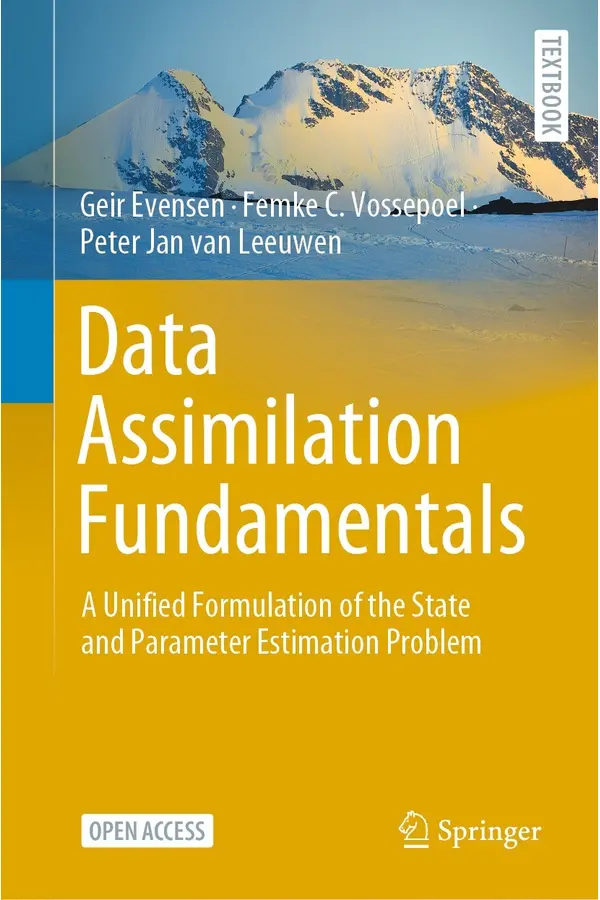
Not rated yetRate this bookData Assimilation Fundamentals: A Unified Formulation of the State and Parameter Estimation Problem develops a common probabilistic framework for combining models and observations. Geir Evensen, Femke C. Vossepoel, and Peter Jan van Leeuwen connect mathematical formulations with numerical examples across twenty-three chapters.
Free reading is available at the official source. Opens in a new tab.
 Free
About this book
Data Assimilation Fundamentals: A Unified Formulation of the State and Parameter Estimation Problem develops a common probabilistic framework for combining models and observations. Geir Evensen, Femke C. Vossepoel, and Peter Jan van Leeuwen connect mathematical formulations with numerical examples across twenty-three chapters.
How to study this book
Keep a notation sheet for state, parameters, observations, operators, and covariance. Derive small scalar or linear cases before studying full algorithms. For each method, record assumptions, approximation, estimated quantity, computational demands, and diagnostic checks; reproduce examples with fixed settings before changing one factor at a time.
Chapter-wise explanations and study tasks
Chapter 1 — Introduction
The introduction frames data assimilation as inference from uncertain models and observations. Distinguish state estimation, parameter estimation, filtering, and smoothing before comparing algorithms. A fitted trajectory is not a complete description of uncertainty.
Study task: Describe a simple estimation problem with unknowns, observations, uncertainty sources, and a clear inference objective.
Chapter 2 — Problem Formulation
Bayesian and recursive formulations connect uncertain inputs, states, measurement errors, assimilation windows, and error propagation. Different formulations retain or marginalize different quantities. Make conditional dependencies explicit before manipulating equations.
Study task: Draw a probabilistic dependency diagram and write the prior, likelihood, and posterior for a small scalar example.
Chapter 3 — Maximum a Posteriori Solution
MAP estimation selects a posterior mode, with Gaussian assumptions leading to familiar objective functions and iterative solutions. Compare a mode with a full posterior distribution. Gauss–Newton approximations require attention to nonlinearity and convergence.
Study task: Derive a scalar Gaussian MAP estimate and explain which features of the posterior a single optimized point does not describe.
Chapter 4 — Strong-Constraint 4DVar
Strong-constraint 4DVar treats the model trajectory as constrained by a perfect-model assumption. The chapter develops variational formulations and related calculations. Identify which uncertainty remains estimable and which is excluded by the formulation.
Study task: Write the objective and constraints for a small time-window problem and explain the role of initial-condition uncertainty.
Chapter 5 — Weak Constraint 4DVar
Weak-constraint formulations admit model error rather than forcing the trajectory to satisfy a perfect model. This changes unknowns, penalties, and computational structure. Examine how the assumed error covariance influences the balance between model evolution and observations.
Study task: Compare strong- and weak-constraint versions of the same conceptual problem, listing additional unknowns and uncertainty assumptions.
Chapter 6 — Kalman Filters and 3DVar
The chapter connects sequential updates and variational analysis within the common framework. Track forecast and analysis means and covariances separately. Distinguish the exact linear-Gaussian result from approximations used outside those assumptions.
Study task: Perform a scalar forecast-and-update calculation and explain how changing observation uncertainty changes the update weight.
Chapter 7 — Randomized-Maximum-Likelihood Sampling
Randomized maximum likelihood uses perturbed optimization problems to generate a sample representation. Compare when the construction reproduces desired statistics with what can change under nonlinearity. Sampling uncertainty and optimization error are separate concerns.
Study task: Outline the logic of a linear test case and specify statistics that would assess whether the generated sample matches the target.
Chapter 8 — Low-Rank Ensemble Methods
Ensemble methods represent uncertainty in a subspace determined by a finite sample. This makes large problems tractable while introducing sampling and rank limitations. Compare the role of the ensemble in representing covariance with the algorithm's update approximation.
Study task: Use a small matrix example to identify the ensemble subspace and explain which directions cannot be represented by its covariance.
Chapter 9 — Fully Nonlinear Data Assimilation
Fully nonlinear methods address inference that cannot be adequately summarized by a Gaussian approximation alone. Consider how methods represent distributions and where computational difficulty enters. A nonlinear model does not guarantee a strongly non-Gaussian posterior, so inspect the actual inference problem.
Study task: Sketch a non-Gaussian posterior and compare what a mean-covariance approximation and a sample representation preserve.
Chapter 10 — Localization and Inflation
Localization and inflation address practical difficulties in finite-ensemble estimation. They modify different aspects of the approximation and require diagnostics rather than automatic application. Compare sampling-related correlations with uncertainty underestimation.
Study task: Design a sensitivity experiment varying localization and inflation separately and specify performance and spread diagnostics.
Chapter 11 — Methods' Summary
The methods summary makes assumptions and relationships easier to compare. Organize methods by what they estimate, how they approximate uncertainty, and the computational structure. Avoid ranking them independently of the problem and data.
Study task: Build a comparison matrix for four methods with assumptions, uncertainty representation, computational needs, and likely limitations.
Chapter 12 — A Kalman Filter with the Roessler Model
The first application uses a dynamical example to make sequential estimation concrete. Compare predicted and updated behaviour and examine the effect of uncertainty assumptions. The example's controlled setting supports understanding but does not prove general performance.
Study task: Reconstruct the experiment's information flow and propose one controlled change to observation frequency or uncertainty.
Chapter 13 — Linear EnKF Update
A linear update isolates ensemble sampling from stronger nonlinear complications. Compare sample-based estimates with the corresponding analytical benchmark. Repeated trials help distinguish systematic behaviour from one fortunate ensemble draw.
Study task: Specify a repeated-trial experiment comparing ensemble sizes and assess mean error, covariance agreement, and variability across runs.
Chapter 14 — EnKF for an Advection Equation
Advection connects a spatially evolving field with observations and ensemble updates. Consider how information propagates through the model and estimated covariance. Evaluate the relationship between observed locations and unobserved parts of the state.
Study task: Draw a space-time observation layout and explain how it affects estimation of an advecting feature.
Chapter 15 — EnKF with the Lorenz Equations
The Lorenz example introduces a nonlinear dynamical setting for ensemble filtering. Compare forecast, update, and uncertainty behaviour over time rather than judging a single analysis. Initial conditions and observation design affect the experiment.
Study task: Define a controlled comparison of two observation configurations using identical model and ensemble settings.
Chapter 16 — 3DVar and SC-4DVar for the Lorenz 63 Model
The chapter compares formulations through observation density, partial observation, window length, and ensemble-method comparisons. Changing several settings simultaneously can obscure the reason for a performance difference. Keep the comparison's information budget explicit.
Study task: Design a one-factor-at-a-time test of assimilation-window length and explain the diagnostics needed to compare the methods fairly.
Chapter 17 — Representer Method with an Ekman-Flow Model
The Ekman-flow example connects the representer approach with a physical model and real measurements. Distinguish model assumptions from data properties and numerical choices. Residuals need interpretation within that combined framework.
Study task: Create a case summary of model, observations, estimated quantities, uncertainty assumptions, and evidence used to assess the result.
Chapter 18 — Comparison of Methods on a Scalar Model
A scalar problem makes posterior shape and algorithmic differences easier to inspect. Compare methods against a common inference target instead of comparing only final fitted values. Small examples can expose limitations hidden in large applications.
Study task: Specify a benchmark posterior and compare two approximate solutions by mode, mean, spread, and representation of asymmetry.
Chapter 19 — Particle Filter for Seismic-Cycle Estimation
Particle filtering is applied to a seismic-cycle estimation problem. Examine how model evolution, observation information, and particle weighting interact. Distinguish the source's controlled estimation example from a guarantee of operational earthquake prediction.
Study task: Map the application workflow and identify diagnostics for particle diversity, weighting, and sensitivity to assumptions.
Chapter 20 — Particle Flow for a Quasi-Geostrophic Model
The particle-flow example examines movement from prior toward posterior information in a spatial dynamical setting. Track the intended target distribution and approximations introduced along the way. Compare computational and statistical diagnostics.
Study task: Prepare a conceptual comparison of particle flow and reweighting, listing how you would assess distributional agreement.
Chapter 21 — EnRML for History Matching Petroleum Models
History matching uses observed behaviour to constrain uncertain model quantities. The chapter connects ensemble optimization with a domain application. A close fit can coexist with non-unique parameters or weak predictions outside the calibration period.
Study task: Separate calibration fit, parameter uncertainty, and predictive checking in a fictional history-matching assessment.
Chapter 22 — ESMDA with a SARS-COV-2 Pandemic Model
The pandemic-model example illustrates parameter estimation through repeated assimilation within an ensemble smoother framework. Model structure and observation assumptions limit interpretation. Treat the example as a historical methodological case, not a current epidemiological forecast.
Study task: Create an assumption audit covering observed quantities, uncertain parameters, model discrepancy, calibration, and out-of-sample checking.
Chapter 23 — Final Summary
The final chapter returns to a unified view of methods and problem formulation. Explain why algorithm choice follows the inference target, uncertainty, and practical constraints. Identify which conclusions are supported by the demonstrations and which require new testing.
Study task: Write a method-selection memo for a new fictional problem and justify the choice against two alternatives.
Applied assignment
Design a reproducible small estimation experiment with a known benchmark, explicit priors and observation errors, two methods, repeated trials where relevant, and accuracy-and-uncertainty diagnostics. Explain failure cases rather than reporting only the best result.
Suggested reading plan
Read Chapters 1–3 for formulation, 4–10 for methods, and 11 for comparison. Work through Chapters 12–18 before selecting a domain application from 19–22; finish with Chapter 23.
Questions for reflection
- What is the target distribution or estimate?
- Which approximation matters most in this example?
- Does a close fit imply credible uncertainty or prediction?
Edition and source notes
Based on the 2022 Springer textbook by Geir Evensen, Femke C. Vossepoel, and Peter Jan van Leeuwen. The guide follows twenty-three chapters, distinguishing mathematical methods from their illustrative applications. Software or linked resources may differ from the publication version; reproduce the stated example settings before extending them.
About access & copyright
This page provides book information and study material. Full-text access is provided by the original publisher or authorised source; a listing does not grant permission to republish the book.
Read our Library Access & Copyright policyExplore the contents
Check the chapters covered in this edition.
Visit the official source
See reading, preview or purchase options.
Save for later
Keep this textbook in your saved collection.
Reader ratings & reviews
Share your thoughts
Your review helps other students choose the right resources.
KEEP LEARNING
Your next great read
Air Pollution Complaints; Family medicine; General practice; Symptoms; Primary care; Prognosis; Diseases; Practice
Morbidity in primary care
View Morbidity in primary care — book agriculture public-private parternship
Wheat Improvement
View Wheat Improvement — book bioinformatics
Systems Biology
View Systems Biology — book Capital Budgeting
Corporate Finance for Long-Term Value
View Corporate Finance for Long-Term Value — book Basic models of the enterprise
Management in a Dynamic Environment
View Management in a Dynamic Environment — book Built Environment
Introduction to Space Syntax in Urban Studies
View Introduction to Space Syntax in Urban Studies — book college
Prose Fiction: An Introduction to the Semiotics of Narrative
View Prose Fiction: An Introduction to the Semiotics of Narrative — book Cultural Rights
Non-Territorial Autonomy
View Non-Territorial Autonomy — book Business enterprises—Finance