
 differential equations
circuit-QEDTextbook
Lecture Notes on Quantum Electrical Circuits
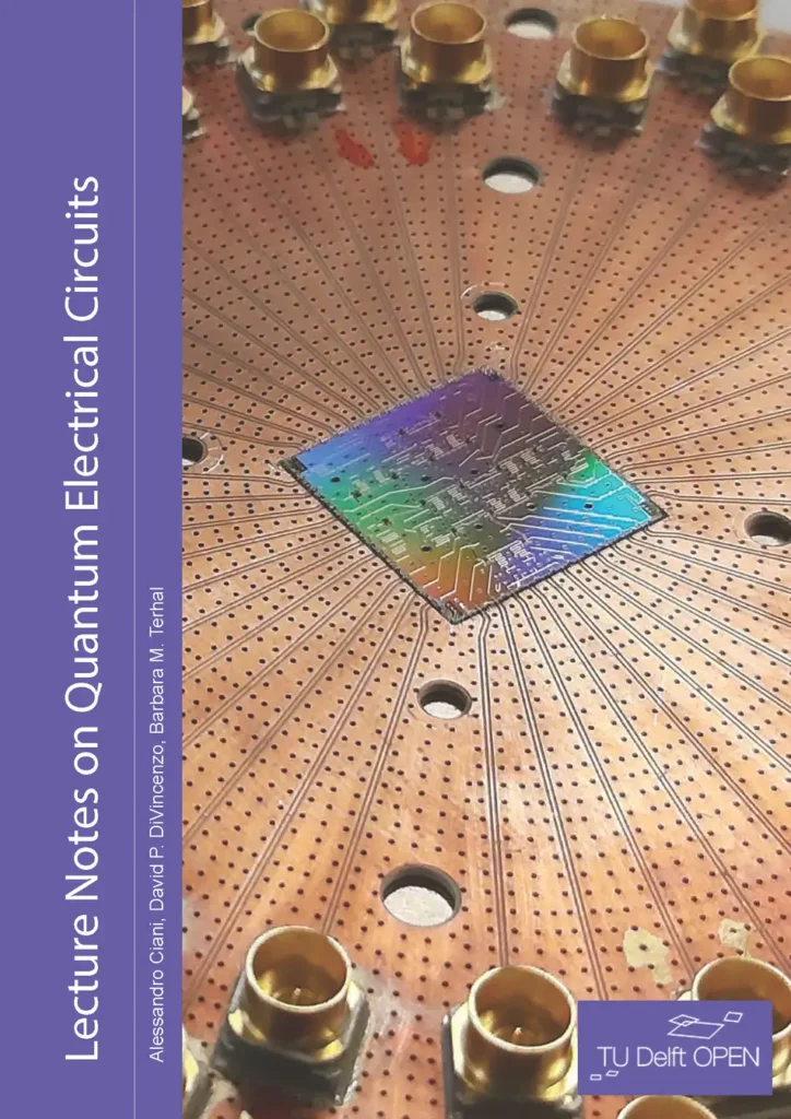
Not rated yetRate this bookLecture Notes on Quantum Electrical Circuits develops the theory needed to model superconducting circuits as quantum systems. Alessandro Ciani, David P. DiVincenzo, and Barbara M. Terhal connect circuit graphs, Lagrangians, canonical variables, and Hamiltonians with qubits, resonators, networks, dissipation, and amplification. This guide follows eight numbered chapters and two mathematical appendices in the linked PDF. It assumes familiarity with linear algebra, classical mechanics, electrical circuits, and introductory quantum theory.
Free reading is available at the official source. Opens in a new tab.
 Free
About this book
Lecture Notes on Quantum Electrical Circuits develops the theory needed to model superconducting circuits as quantum systems. Alessandro Ciani, David P. DiVincenzo, and Barbara M. Terhal connect circuit graphs, Lagrangians, canonical variables, and Hamiltonians with qubits, resonators, networks, dissipation, and amplification. This guide follows eight numbered chapters and two mathematical appendices in the linked PDF. It assumes familiarity with linear algebra, classical mechanics, electrical circuits, and introductory quantum theory.
Chapter-wise summaries and study tasks
Chapter 1. Introduction
The introduction establishes the scope and prerequisites of circuit quantization. A superconducting device is described through a physical circuit, a choice of variables, and a quantum model whose approximations determine its usefulness. Classical circuit intuition and quantum mechanics must be connected rather than applied as unrelated stages. The notes emphasize systematic derivation and examples that expose conditions under which familiar shortcuts fail.
Keep a hierarchy of descriptions: components and connections, classical energy or equations, canonical variables, operators, and any reduced effective model. At each transition ask which degrees of freedom and interactions are retained. This helps distinguish a convenient two-level approximation from the full circuit’s spectrum.
Study task. Choose an LC circuit as a running example and list the information required at each modeling stage. Identify which additional assumptions would be needed before calling a general circuit a qubit.
Chapter 2. Lagrangians and Hamiltonians for electrical circuits
Branch voltages and fluxes support an energy-based description of inductive and capacitive elements. Circuit graphs impose conservation relationships, while a suitable coordinate choice leads to a Lagrangian and Hamiltonian. The LC oscillator provides a basic quantization example; Josephson elements add nonlinear structure and support the Cooper-pair-box model. Mutual inductance, ideal transformers, sources, and external fluxes require careful treatment rather than arbitrary insertion into a familiar formula.
Canonical charge follows from the Lagrangian and need not equal every casually labeled physical branch charge. Time-dependent external fluxes and superconducting constraints add further conditions. Verify dimensions and conservation relationships before promoting variables to operators.
Study task. Derive the energy and canonical variables of a simple circuit, then add one coupling or source. Explain how the graph constraints and variable definitions change before writing the revised Hamiltonian.
Chapter 3. Applying canonical quantization
Applying canonical quantization requires independent coordinates and a well-defined classical formulation. The capacitance matrix’s invertibility and the structure of constraints affect whether a naive Legendre transform is valid. Capacitive interactions can appear nonlocal in the Hamiltonian through matrix inversion, so graphical proximity alone does not determine the form of every coupling. Examples involving flux qubits, fluxonium, protected-circuit ideas, and other arrangements test the procedure.
Symmetries can organize states and forbid transitions under specified operators. A missing matrix element is therefore a statement about a symmetry and coupling mechanism, not a universal impossibility of exciting the device. Examine which assumptions remain valid after a circuit modification.
Study task. Compare a regular and a constrained circuit formulation, checking the capacitance matrix. For a symmetric example, identify the relevant symmetry and explain which perturbation could permit a previously forbidden transition.
Chapter 4. The transmon qubit, resonators and their coupling
The Cooper-pair-box Hamiltonian and its spectrum lead into the transmon regime and an anharmonic approximation. Reduced sensitivity to some fluctuations comes with tradeoffs in level structure and control. Driving a transmon, transmission lines, boundary conditions, and resonator modes connect the device with its electromagnetic environment. Input–output and Heisenberg–Langevin descriptions address coupling to propagating fields. Capacitive qubit–resonator coupling and perturbative tools support effective models.
A two-level truncation, weak-coupling approximation, or dispersive treatment needs a scale comparison. The presence of a coupling term does not justify using the same reduced Hamiltonian in every parameter regime. Track frequencies, detunings, anharmonicity, and coupling strengths.
Study task. Draw a scale table for a hypothetical transmon–resonator system. Explain when a two-level or dispersive approximation might be defensible and identify a parameter change that would require reconsidering it.
Chapter 5. Linear networks and black-box quantization
Linear-network theory provides a way to characterize complex circuits through ports, response functions, and scattering descriptions. Laplace and Fourier representations connect dynamical equations with frequency-dependent behavior. Black-box quantization uses the linearized environment and modal information to construct a quantum model, with energy-participation and single-port approaches offering related tools. Lossy networks and the QuCAT example extend the treatment toward practical calculation.
A measured or simulated response is useful only with clear port definitions and normalization. Linearization organizes the problem but does not remove nonlinear effects; those must be incorporated consistently into the chosen approximation. Compare the reduced model with the network quantities used to derive it.
Study task. Map a multi-element circuit into ports and a linearized response. Explain what information is needed to recover modes and nonlinear corrections, then identify an independent check on a software-generated result.
Chapter 6. Nonreciprocity
Nonreciprocity concerns direction-dependent response and cannot be inferred simply from a circuit having several ports. The circulator and gyrator provide concrete devices for examining port relationships and conservation. Their admittance or scattering descriptions must be interpreted with consistent conventions. The notes develop a Lagrangian and Hamiltonian treatment of a gyrator and compare aspects of its behavior with a magnetic-field analogy.
An analogy clarifies a mathematical structure without making every physical mechanism identical. Separate reciprocity, passivity, and loss rather than using them interchangeably. Check power accounting and the chosen port definitions when interpreting an ideal nonreciprocal element.
Study task. Compare reciprocal and nonreciprocal port-response matrices under the source’s conventions. Trace power through an ideal device and explain which property distinguishes directionality from dissipation.
Chapter 7. Noise, or all that can go wrong
Noise and loss make an isolated Hamiltonian an incomplete account of device behavior. A Lindblad master-equation model introduces dissipative dynamics under assumptions that must fit the environment and timescales. A lossy branch provides a circuit-specific example. Sensitivity to parameter fluctuations, flux sweet spots, and built-in protection connect design with particular noise mechanisms.
Protection is conditional: reducing first-order sensitivity to one variable does not establish immunity to all errors or remove relaxation channels. Distinguish coherent dynamics, energy relaxation, and loss of phase coherence. A useful comparison identifies the coupling operator, environmental assumption, and observable affected.
Study task. For a fictional qubit circuit, distinguish a Hamiltonian parameter fluctuation from a dissipative channel. Explain what a sweet spot suppresses locally and list a noise mechanism that remains outside that protection claim.
Chapter 8. Models of superconducting amplifiers
The amplifier chapter is organized around models and exercises that extend the earlier circuit and mode descriptions. Amplification requires accounting for driving, coupling, gain, and the additional fluctuations associated with an open quantum system. A classical increase in signal amplitude is not a complete explanation of quantum amplifier behavior. Use the exercises to identify the physical interactions and approximations behind an effective model.
Keep input, output, and internal modes distinct, and state whether an analysis treats particular quadratures or a more general signal. Stability and the operating regime matter when interpreting a calculated gain. A model valid near a selected operating point should not be extrapolated without checking its assumptions.
Study task. Reconstruct one amplifier exercise from its physical interactions to its reduced equations. Identify the energy source, input–output relation, and assumptions needed before interpreting gain or noise.
Appendix A. A review of canonical quantization
The first appendix reviews the classical foundations used throughout the text: action, gauge considerations, the Legendre transformation, Poisson brackets, and canonical quantization. It connects equations of motion with the selection of conjugate variables and the passage to operators. These steps help explain why a circuit Hamiltonian should be derived from a consistent formulation rather than guessed from component names.
Coordinate or gauge choices can change a representation without changing the physical prediction when handled consistently. Verify which quantities are independent and which constraints have already been applied. The review is especially useful when two derivations appear different but aim to describe the same system.
Study task. Derive a simple Hamiltonian from a Lagrangian and identify the conjugate pair. Compare two consistent representations and explain which prediction should remain invariant despite changes in intermediate expressions.
Appendix B. Harmonic systems and beyond
The second appendix develops normal modes, diagonalization, and reductions of coupled harmonic systems. Eliminating high-frequency modes requires a separation of scales and an explicit approximation, illustrated through a Born–Oppenheimer-style argument. Cauer-related network construction connects response descriptions with circuit realization, while a shunted LC example shows how a small admittance modifies behavior.
A mode omitted from a reduced model can still shift parameters or generate effective interactions. The goal is not simply to delete inconvenient variables but to estimate their influence in the regime being studied. Compare the reduced spectrum or response with the full model where possible.
Study task. Diagonalize a small coupled harmonic system and compare its exact modes with a reduced description. Vary the scale separation and identify where the eliminated mode’s effects become too large to neglect.
How to study this book
- Track circuit graph, independent coordinates, classical energy, conjugate variables, and operator model in a single derivation record.
- Check matrix dimensions, units, constraints, and signs before using numerical diagonalization.
- List the scale assumptions behind every linearization, perturbative expansion, mode elimination, and level truncation.
- Solve the source’s derivation and computational exercises, comparing simplified models with small full-system calculations.
- Treat software and device examples as source-specific implementations; verify conventions and current documentation when reproducing them.
Questions for reflection
- Which step introduces an approximation rather than an exact change of variables?
- How could a symmetry or constraint invalidate a convenient transition or coordinate assumption?
- What physical channel remains outside a claimed protection mechanism?
Source edition and coverage
This guide covers the linked PDF’s eight numbered chapters and appendices on canonical quantization and harmonic systems. It follows the supplied circuit-theory content rather than serving as a laboratory construction or device-calibration manual. These are original study explanations and learning tasks. Read the complete book at the official source.
About access & copyright
This page provides book information and study material. Full-text access is provided by the original publisher or authorised source; a listing does not grant permission to republish the book.
Read our Library Access & Copyright policyExplore the contents
Check the chapters covered in this edition.
Visit the official source
See reading, preview or purchase options.
Save for later
Keep this textbook in your saved collection.
Reader ratings & reviews
Share your thoughts
Your review helps other students choose the right resources.
KEEP LEARNING
Your next great read
differential equations connected networks
Network quality control
View Network quality control — book Psychology
Introduction to Psychology
View Introduction to Psychology — book citizen science
Library Infrastructures & Citizen Science: A Guide
View Library Infrastructures & Citizen Science: A Guide — book Data Driven Innovation
Legal challenges in Data Driven Innovation
View Legal challenges in Data Driven Innovation — book Humanities
Writing Guide with Handbook
View Writing Guide with Handbook — book Dynamics
Introductory Dynamics: 2D Kinematics and Kinetics of Point Masses and Rigid Bodies, Edition 1.1
View Introductory Dynamics: 2D Kinematics and Kinetics of Point Masses and Rigid Bodies, Edition 1.1 — book Humanities
World History, Volume 2: from 1400
View World History, Volume 2: from 1400 — book Business
Workplace Software and Skills
View Workplace Software and Skills — book Humanities