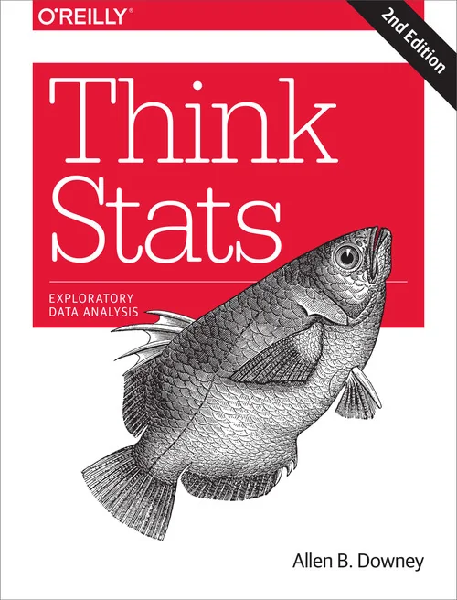
Think Stats: Probability and Statistics for Programmers

Think Stats uses executable Python analysis to connect statistical questions with real data. The library's catalog title, Probability and Statistics for Programmers, points to the second-edition PDF titled Exploratory Data Analysis in Python, version 2.2.1. This guide follows that file's fourteen chapters rather than the newer third edition. Survey data provide a continuing case, but the main lessons concern measurement, distributions, relationships, uncertainty, and the limits of inference. Historical datasets and software examples are learning material, not present-day population estimates or a promise that every original API call will run unchanged.

Chapter-by-chapter summaries

Chapter 1: Exploratory data analysis

A statistical investigation begins with a question that can be connected to observable variables. Downey introduces National Survey of Family Growth records, data import, DataFrames, transformations, validation, and interpretation. Data cleaning is part of the argument because special codes, missing values, and measurement conventions determine what a calculation describes. Reproducing a published number is not enough if the selected records or units differ. The opening example encourages readers to examine an informal claim by specifying groups and an outcome, then inspect whether the available data can support the proposed comparison.

Study task. Create a data dictionary and verify a transformation with hand-checked records before comparing two groups.

Chapter 2: Distributions

Histograms reveal how observations are distributed and make outliers and group differences visible before they are compressed into summary statistics. Mean, variance, and effect size answer different questions, and a small difference in means can coexist with substantial overlap between groups. The chapter emphasizes reporting what a result means in its original units. Unusual observations need investigation rather than automatic deletion; an apparent outlier might be an encoding mistake or a genuine part of the phenomenon. Distributional thinking establishes the foundation for later probability models and helps keep a striking anecdote from standing in for the full dataset.

Study task. Compare group histograms and report the difference in means alongside variability and a practical interpretation of effect size.

Chapter 3: Probability mass functions

A probability mass function converts counts into normalized probabilities, making distributions comparable even when sample sizes differ. The class-size paradox illustrates how the way people encounter groups can produce size-biased observations. A typical student's experience can differ from the typical class without either calculation being arithmetically wrong. The chapter also develops DataFrame indexing as a means of expressing a precise selection. Identify the unit being sampled and the weighting implied by the question before interpreting an average. This is an early demonstration that a data representation and a sampling mechanism must be understood together.

Study task. Calculate class-size distributions from both class and student perspectives and explain the weighting responsible for their difference.

Chapter 4: Cumulative distribution functions

A cumulative distribution function answers how much probability lies at or below a value. It provides a useful alternative when PMFs become visually crowded and supports percentiles, medians, and percentile-based measures of spread. Comparing CDFs highlights where groups differ across a distribution rather than at one average. Inverse use of the CDF also connects probability models with random generation. Percentile rank and the value associated with a percentile are related but distinct questions. Careful axis interpretation prevents confusion between a measurement, a probability, and the fraction of observations satisfying a threshold.

Study task. Plot two empirical CDFs, compare their medians and tails, and use selected percentiles to describe differences obscured by their means.

Chapter 5: Modeling distributions

Empirical distributions describe observed data, while analytic distributions provide simplified mathematical models. Exponential, normal, lognormal, and Pareto examples demonstrate why different mechanisms and scales call for different shapes. Diagnostic plots can expose where a proposed model fits poorly, especially in the tails. A model's convenience does not establish that its assumptions hold. Distinguish fitting a parameter from validating a family of distributions, and avoid extrapolating far beyond the evidence because a straight line appears in a transformed plot. The chapter prepares readers to use models as explicit approximations rather than replacements for checking the observations.

Study task. Fit two candidate distribution families to a variable and compare their central fit and tail behavior using appropriate plots.

Chapter 6: Probability density functions

Density extends distributional reasoning to continuous measurements. The height of a density curve is not itself the probability of an exact value; probability is associated with area over an interval. Kernel density estimation supplies a smooth empirical representation whose appearance depends on the smoothing choice. The chapter connects density, cumulative probability, moments, skewness, and random sampling. Keep the mathematical distribution separate from both a finite sample and the visualization used to display it. Different representations can emphasize different features without changing the underlying question, but smoothing can hide structure or create a misleading impression of precision.

Study task. Compare a histogram, CDF, and density estimate of one variable, varying bandwidth and explaining which conclusions remain stable.

Chapter 7: Relationships between variables

Scatterplots, conditional distributions, covariance, and correlation provide complementary ways to investigate paired observations. Visualization matters because a numerical association can conceal nonlinearity, outliers, or changing spread. Pearson correlation emphasizes a linear relationship, while rank-based analysis asks a different question about ordering. Neither establishes causation. Overplotting can also make a dense region look like only a few points, so the display method should match the data volume and measurement precision. Interpret a relationship in the context of both variables and the sampling process rather than assigning meaning to a coefficient in isolation.

Study task. Use plots and both linear and rank correlations to examine one pair of variables, then identify a plausible noncausal explanation.

Chapter 8: Estimation

An estimator is a rule for learning an unknown quantity from a sample. Repeated sampling or simulation reveals how that rule behaves, introducing bias, variability, standard error, and confidence intervals. These properties differ: an estimator can be unbiased yet too variable for a useful decision. The chapter connects practical resampling with the sampling distribution behind uncertainty statements. A confidence interval depends on a procedure and assumptions; it is not a guarantee about a particular observed interval. Simulation becomes a way to investigate whether a method performs as intended under a model whose true value is known.

Study task. Simulate repeated samples from a known distribution and compare the bias, standard error, and interval coverage of two estimators.

Chapter 9: Hypothesis testing

Hypothesis testing compares an observed statistic with what a specified null model would typically produce. Permutation and simulation make the logic concrete before more specialized procedures are considered. A p-value describes extremeness under that model, not the probability that the null hypothesis is true. The chapter discusses differences, correlations, chi-squared comparisons, errors, power, and replication. Statistical significance must be separated from effect size and the quality of the research design. Choosing a statistic after searching many possibilities changes the interpretation, so an analysis should state its question and decision process clearly.

Study task. Implement a permutation test with a stated null hypothesis and statistic, and report the observed effect separately from its simulated p-value.

Chapter 10: Linear least squares

A fitted line summarizes a conditional relationship by minimizing squared residuals. Slope and intercept require interpretation in the variables' units, while residual plots reveal patterns the fitted line leaves unexplained. The chapter develops implementation, estimation, goodness of fit, model testing, and weighted resampling. A high fit statistic does not establish causality or justify extrapolation outside the observed range. Survey weights further illustrate that the target population and the observed sample need not have the same representation. A useful regression report therefore explains the model, uncertainty, diagnostics, and intended domain of prediction.

Study task. Fit a line, inspect residuals, and explain how a prediction changes when survey weighting or the fitted data range changes.

Chapter 11: Regression

Multiple regression extends the model to several predictors, making each coefficient conditional on the others included. Nonlinear terms and logistic regression show that different outcomes and relationships need different specifications. Searching many predictors can produce an apparently persuasive model that does not generalize. The chapter's data-mining discussion reinforces the need for substantive reasoning and independent evaluation. Distinguish explanation, adjustment, and prediction: they are not interchangeable goals. In logistic regression, interpret changes through probabilities or odds carefully rather than treating a coefficient as a direct percentage-point change in the outcome.

Study task. Compare a simple and adjusted model, then evaluate predictive performance on held-out observations and explain any coefficient change.

Chapter 12: Time series analysis

Time-ordered observations carry dependence that ordinary independent-sample reasoning can miss. The chapter develops import and cleaning, regression, moving averages, missing-value handling, serial correlation, autocorrelation, and forecasting. A trend and a short-term fluctuation describe different components, while smoothing alters what can be seen. Interpolation across missing periods makes an assumption about unobserved behavior. Forecast evaluation should respect temporal order, because training on future observations can leak information into a supposed prediction. The practical lesson is to treat time as part of the data-generating structure rather than merely another plotting label.

Study task. Separate trend and residual variation in a series, inspect autocorrelation, and assess a forecast using later observations reserved in advance.

Chapter 13: Survival analysis

Survival analysis studies time until an event while accounting for observations whose event time is not yet known. Such censoring is information about having survived at least to a point, not a reason to discard a record. Survival curves and hazard functions answer different questions, and Kaplan-Meier estimation uses the changing population at risk. Marriage examples illustrate cohort comparisons, uncertainty, remaining lifetime, and the danger of extrapolating an unfinished curve. The method's validity depends on how observation ends and whether censoring is informative. Always define the event and time origin before interpreting a curve.

Study task. Build a small censored dataset by hand and trace the risk set and survival estimate at each observed event time.

Chapter 14: Analytic methods

The final chapter compares computational inference with mathematical approximations involving normal distributions and the central limit theorem. Sampling distributions explain why some statistics become approximately normal under suitable conditions, while simulation helps test when that approximation is useful. Correlation and chi-squared examples connect the new calculations with earlier computational tests. An analytic result is only as applicable as its assumptions about independence, sample size, and distributional behavior. Rather than treating simulation and formulas as competing camps, use agreement and disagreement between them to diagnose an analysis and understand the source of its uncertainty.

Study task. Compare a resampling-based uncertainty calculation with an analytic approximation and investigate a setting where their agreement deteriorates.

Study instructions

1. Preserve an untouched copy of each dataset and record the meaning of special codes, missing values, units, and survey weights.
2. Begin each analysis with a question, observational unit, target population, and proposed comparison.
3. Use distributions and diagnostic plots before reducing results to a coefficient or p-value.
4. Keep effect size, uncertainty, model assumptions, and causal interpretation in separate sentences when reporting findings.
5. Complete an original reproducible analysis that includes data validation, at least two distribution views, a model check, and a statement of limitations.

Questions for reflection

• How does a sampling mechanism change the meaning of a typical observation?
• When can an interval look precise while describing the wrong target?
• What evidence beyond an association would be needed for a causal claim?

Sources and coverage

This original study guide follows the linked source edition and its complete main chapter sequence. It explains the ideas in new wording and adds reading tasks; it does not replace the textbook, reproduce its exercises, or supply an answer key. Publisher and book source; Complete source PDF.