
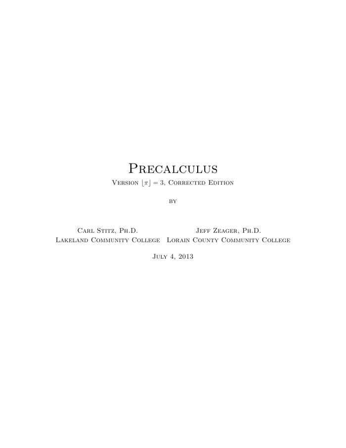
 Calculus
Geometry and TrigonometryTextbook
College Trigonometry
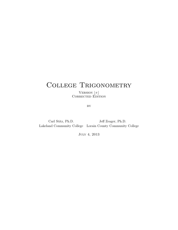
Not rated yetRate this bookCollege Trigonometry by Carl Stitz and Jeff Zeager develops circular functions and their applications through exact reasoning, graphs, algebra, and geometric interpretation. The linked file is the July 4, 2013 corrected edition, Version floor(pi), and contains 398 PDF pages. It retains Chapters 10 and 11 from the authors' larger Precalculus text, so the numbering begins at 10 rather than 1. This guide covers all sixteen main sections within those two chapters. Learners should already be comfortable with algebra, functions, equations, and coordinate geometry. The original title page from the linked PDF is used as the cover so the image matches this edition rather than the newer edition pictured in the catalog.
Read on the publisher’s website. Opens in a new tab.
 Free
About this book
College Trigonometry by Carl Stitz and Jeff Zeager develops circular functions and their applications through exact reasoning, graphs, algebra, and geometric interpretation. The linked file is the July 4, 2013 corrected edition, Version floor(pi), and contains 398 PDF pages. It retains Chapters 10 and 11 from the authors' larger Precalculus text, so the numbering begins at 10 rather than 1. This guide covers all sixteen main sections within those two chapters. Learners should already be comfortable with algebra, functions, equations, and coordinate geometry. The original title page from the linked PDF is used as the cover so the image matches this edition rather than the newer edition pictured in the catalog.
Book summary
About this book
College Trigonometry by Carl Stitz and Jeff Zeager develops circular functions and their applications through exact reasoning, graphs, algebra, and geometric interpretation. The linked file is the July 4, 2013 corrected edition, Version floor(pi), and contains 398 PDF pages. It retains Chapters 10 and 11 from the authors' larger Precalculus text, so the numbering begins at 10 rather than 1. This guide covers all sixteen main sections within those two chapters. Learners should already be comfortable with algebra, functions, equations, and coordinate geometry. The original title page from the linked PDF is used as the cover so the image matches this edition rather than the newer edition pictured in the catalog.
Chapter-by-chapter study guide
Chapter 10 overview: Foundations of Trigonometry
The chapter connects angle measurement, coordinates, circular functions, identities, graphs, inverses, and equations. The unit circle supplies the geometric foundation from which signs, exact values, and periodicity can be understood. Algebra then extends those relationships without replacing their meaning. A recurring distinction is between a function's definition, an identity valid across a common domain, and an equation satisfied by particular angles. Studying the chapter as a sequence helps prevent isolated formula memorization, because later transformations and solution methods depend on the earlier geometric relationships.
Study application: Create a concept map linking angle, unit-circle point, sine, cosine, tangent, graph, and inverse. Add an example showing where a function is undefined and why.
Section 10.1: Angles and Their Measure
Degree and radian measures describe the same rotation using different units. Radians connect angle with arc length through a ratio, making them especially useful in circular motion and later calculus. Coterminal angles share a terminal side but differ by full rotations. Reference angles help locate related acute-angle geometry, while signed angles distinguish direction. Arc length, sector area, angular speed, and linear speed require consistent units; formulas using radians cannot be applied blindly to degree values. A diagram should accompany the calculation to establish radius, direction, and the relevant interval.
Study application: Convert a signed angle between degrees and radians, find a positive coterminal angle, and compute arc length on a stated circle. Explain how doubling radius changes linear speed at a fixed angular speed.
Section 10.2: The Unit Circle — Cosine and Sine
A point on the unit circle gives cosine as its horizontal coordinate and sine as its vertical coordinate. Symmetry and reference angles extend familiar first-quadrant values to the whole circle. The identity involving the squares of sine and cosine follows from the circle equation, while signs depend on quadrant. Scaling a unit-circle picture connects the circular definition with right-triangle ratios and coordinates on any circle. Exact values carry relationships that decimal approximations can conceal. A calculator result is a check, not a substitute for identifying quadrant and geometry.
Study application: Derive exact sine and cosine values for related angles in all four quadrants from one reference triangle. Verify their signs and the unit-circle identity without decimal approximations.
Section 10.3: The Six Circular Functions and Fundamental Identities
Tangent, cotangent, secant, and cosecant extend sine and cosine through quotient and reciprocal relationships. Their domains follow from denominators: a reciprocal or quotient is undefined where the relevant quantity is zero. Fundamental identities allow one function value and quadrant information to determine others, but signs must be justified. Relationships valid for all admissible angles differ from isolated numerical equalities. Keeping definitions visible reduces the number of formulas that must be memorized independently and makes domain restrictions easier to track.
Study application: Given one trigonometric value and a quadrant, determine the remaining five values exactly. Identify all excluded angles for a chosen quotient function and explain the geometric reason.
Section 10.4: Trigonometric Identities
Identity work uses fundamental relationships and angle formulas to transform expressions across a shared domain. Sum, difference, double-angle, and related formulas connect values that are not directly familiar. A valid verification preserves meaning at each step; assuming the desired equality or dividing by an expression that may be zero can invalidate an argument. Simplification is goal-dependent: a product, sum, or single-function form may be useful for different purposes. Domain conditions remain part of the statement even when a transformed expression appears simpler.
Study application: Verify an identity by transforming one side, annotating the rule used at each step. Then use an angle-sum or difference formula to obtain an exact unfamiliar value and check its sign geometrically.
Section 10.5: Graphs of the Trigonometric Functions
Graphs connect periodic behavior with function definitions. Sine and cosine have bounded ranges and identifiable amplitudes, periods, midlines, and phase shifts. Tangent and cotangent have different periods and asymptotes, while secant and cosecant are organized around the zeros and extrema of the corresponding reciprocal functions. A horizontal scale factor changes the period, and horizontal translation must be read from a correctly factored argument. Plotting a few arbitrary points can miss essential structure, so key points and asymptotes should be established first.
Study application: Sketch a transformed sinusoid from its parameters and label one full period. Compare it with a transformed tangent graph, explaining why amplitude is not a suitable descriptor for the tangent function.
Section 10.6: The Inverse Trigonometric Functions
Periodic trigonometric functions need domain restrictions before they have inverse functions. Principal-value ranges make the inverse single-valued, so an inverse result may differ from an original angle outside the restricted interval. Compositions therefore require attention to the allowed input and output ranges. Inverse notation means functional reversal, not a reciprocal. The text discusses alternative conventions for inverse secant and cosecant, making it important to state the convention used. Solving a trigonometric equation often requires additional angles beyond the principal inverse value.
Study application: Evaluate an inverse composition using a diagram and the principal range. Then explain why taking inverse sine of a sine value does not always return the original angle.
Section 10.7: Trigonometric Equations and Inequalities
Equations ask which angles satisfy a relationship; inequalities ask which intervals do. Factoring, identities, substitutions, and inverse functions can simplify the task, but each transformation must preserve or later check the solution set. Dividing by a trigonometric expression can lose solutions, while squaring can add extraneous ones. Periodicity extends a solution from a reference interval into a general family. Sign charts and graphs help with inequalities, including open endpoints where a function is undefined. State whether the requested answer is a finite interval list or a general solution.
Study application: Solve an equation that factors into two trigonometric terms without dividing either away. Check each family in the original equation and then restrict the answer to a specified interval.
Chapter 11 overview: Applications of Trigonometry
Applications extend the foundational ideas to periodic models, non-right triangles, polar descriptions, complex numbers, and vector geometry. The appropriate method depends on the information provided and the representation best suited to the problem. A correct computation can still answer the wrong question if angle conventions, coordinate choices, or physical restrictions are ignored. This chapter is especially useful preparation for calculus, physics, and engineering because it connects formulas with direction, motion, and geometry. Each model should include interpretation and a check for alternative solutions.
Study application: Choose one periodic, one triangle, and one vector problem. For each, explain why its chosen representation is useful before performing any calculation.
Section 11.1: Applications of Sinusoids
Sinusoidal models describe repeated variation through amplitude, midline, period, and phase. These parameters connect observed extremes and timing with a formula. Harmonic motion adds physical meaning to displacement and cycle length. Several formulas can describe the same behavior because sine and cosine differ by a phase shift and periodic arguments are nonunique. Fitting a curve does not prove that every future observation will follow it; the model's assumptions and observation range matter. Units must be consistent when frequency or angular frequency is introduced.
Study application: Use a maximum, minimum, and cycle duration to construct a sinusoidal model. Predict a time at which a target value occurs and explain why there may be more than one answer per cycle.
Section 11.2: The Law of Sines
The Law of Sines relates side lengths to the sines of opposite angles and is useful when an opposite side–angle pair is known. The ambiguous side–side–angle case may produce no triangle, one triangle, or two triangles. An inverse-sine calculation supplies only a principal angle, so the supplementary possibility needs examination. Angle sums, side–angle ordering, and the original measurements provide consistency checks. Not every triangle problem has enough information for a unique answer, and numerical rounding should be delayed until the geometry is settled.
Study application: Choose side–side–angle data that permit two triangles. Find both possibilities, check their angle sums and side ordering, and explain why the first calculator angle alone is incomplete.
Section 11.3: The Law of Cosines
The Law of Cosines connects three sides with an included angle and extends the Pythagorean relationship beyond right triangles. It is especially useful for side–angle–side or side–side–side information. Once enough information is known, another triangle relationship can complete the solution, but the choice should avoid unnecessary ambiguity. Computation needs parentheses, consistent units, and a plausible inverse-cosine input. Area formulas connect the resulting geometry with practical measurement. A sketch is a useful check even when it is not drawn to scale.
Study application: Solve a triangle from three side lengths after checking the triangle inequality. Identify its largest angle and confirm that it lies opposite the longest side.
Section 11.4: Polar Coordinates
Polar coordinates locate a point using a directed distance and an angle rather than horizontal and vertical components. Representations are nonunique: adding full rotations or reversing the radius with an adjusted angle can describe the same location. Conversion uses trigonometric relationships, but recovering an angle from a tangent ratio requires quadrant information. The origin has no unique angle. Polar descriptions are natural when distance from a center and direction are more meaningful than rectangular displacement.
Study application: Represent one point using two positive-radius forms and one negative-radius form. Convert it to rectangular coordinates and explain how quadrant information prevents an inverse-tangent error.
Section 11.5: Graphs of Polar Equations
Polar graphs are traced as the angle changes, and negative radii can create behavior that a rectangular-style plotting habit misses. Symmetry tests, zeros of the radius, maximum distances, and strategic angles help reveal shape. Familiar curves include circles and several families with loops or petals. One geometric point can be reached at more than one parameter value, so tracing intervals matter. The graph of a polar equation describes a set of points rather than an ordinary single-valued function of horizontal position.
Study application: Make a table for a polar curve over a suitable angle interval. Mark where the radius changes sign and explain how that affects the plotted points and the completed trace.
Section 11.6: Hooked on Conics Again
Conics can be described in polar form using a focus, directrix, eccentricity, and a consistent orientation. The same geometric curve may have quite different-looking rectangular and polar equations. Eccentricity distinguishes ellipse, parabola, and hyperbola, while denominator signs and trigonometric choices affect placement. Recognizing parameters through geometry is safer than memorizing one formula without its convention. Converting representations can reveal different features, such as a center in rectangular form or a focus-based description in polar form.
Study application: Classify a polar conic by eccentricity and identify its focus/directrix convention. Sketch its orientation and check one point rather than relying on the equation's appearance alone.
Section 11.7: Polar Form of Complex Numbers
A complex number can be represented by magnitude and argument, linking algebra with the plane. Multiplication combines magnitudes and adds arguments, while division subtracts arguments under appropriate nonzero conditions. De Moivre's theorem extends the pattern to integer powers. Finding roots requires all distinct arguments distributed around the circle, not only one principal root. Equivalent arguments explain why care is needed when listing solutions. The connection with polar geometry turns lengthy rectangular calculations into organized magnitude-and-angle reasoning.
Study application: Find every cube root of a nonzero complex number in polar form. Plot them and explain why they are equally spaced, then verify one root by cubing it.
Section 11.8: Vectors
Vectors represent magnitude and direction independently of the point at which an arrow is drawn. Components support addition, subtraction, and scalar multiplication, connecting geometric motion with algebra. A unit vector has magnitude one and describes direction, while a zero vector has no unique direction. Applications include displacement, velocity, and forces, each requiring its own units and interpretation. The magnitude of a sum is generally not the sum of magnitudes because directions matter. Drawing a head-to-tail or parallelogram picture helps check component calculations.
Study application: Combine two directed displacements by components and compare the magnitude of the resultant with total distance traveled. Explain physically why those quantities differ.
Section 11.9: The Dot Product and Projection
The dot product relates component calculations with the angle between vectors. It supports tests of perpendicularity, angle calculations, and scalar or vector projection. Projection identifies the part of one vector in a specified direction and is different from simply comparing magnitudes. A negative dot product indicates an obtuse directional relationship under the usual nonzero-vector interpretation. Work applications combine force with displacement, so only the relevant directional component contributes. Distinguish the scalar dot product from the vector produced by a projection formula.
Study application: Compute an angle and a vector projection from two nonzero vectors. Check that the projection lies in the target direction and that the remaining component is perpendicular to it.
Study instructions
- Review function notation, algebra, factoring, and coordinate geometry before beginning. Keep the source's original Chapter 10–11 numbering in your notes.
- Build exact values from the unit circle and symmetry before using a calculator. Label every angle unit and check calculator mode.
- Separate identities, inverse evaluations, equations, and inequalities; each asks a different kind of question and needs a different final answer.
- Record excluded values before dividing, taking reciprocals, or manipulating an equation. Check solutions after squaring or using inverse functions.
- For applications, draw the geometry, identify given information, choose a method, and examine possible alternative solutions before rounding.
- Compare rectangular, polar, complex, and vector representations to see which makes the relevant relationship simplest.
- Use the section answer sets after a complete attempt. Keep an error log focused on quadrant, domain, periodicity, ambiguity, and units.
Questions for reflection
- Why is inverse sine not a complete solver for every sine equation?
- How can side–side–angle information determine two triangles?
- Why are polar coordinates nonunique?
- What geometric operation corresponds to multiplying complex numbers?
- How does projection differ from vector magnitude?
Sources and edition coverage
Coverage follows the July 4, 2013 corrected PDF, Version floor(pi), including Chapter 10's seven sections and Chapter 11's nine sections. The separate trigonometry book retains the larger Precalculus volume's numbering and printed page numbers. The original linked PDF title page replaces the catalog's newer-edition artwork. The catalog's 2011 date is corrected here to the linked 2013 edition. This is an original study guide. Read the linked textbook for its full explanations, evidence, worked examples, exercises, and references. The study applications above are new practice suggestions, not quoted textbook exercises.
About access & copyright
This page provides book information and study material. Full-text access is provided by the original publisher or authorised source; a listing does not grant permission to republish the book.
Read our Library Access & Copyright policyExplore the contents
Check the chapters covered in this edition.
Visit the official source
See reading, preview or purchase options.
Save for later
Keep this textbook in your saved collection.
Reader ratings & reviews
Share your thoughts
Your review helps other students choose the right resources.
KEEP LEARNING
Your next great read
Calculus Calculus
Whitman Calculus
View Whitman Calculus — book Calculus
Vector Calculus
View Vector Calculus — book Analysis
Basic Analysis: Introduction to Real Analysis, Volume I
View Basic Analysis: Introduction to Real Analysis, Volume I — book Calculus
 for the Life Sciences: A Modeling Approach, Volume 2
View Calculus for the Life Sciences: A Modeling Approach, Volume 2 — book Applied
Introductory Statistics
View Introductory Statistics — book Applied
 Discrete Structures
View Applied Discrete Structures — book Calculus
Precalculus
View Precalculus — book Algebra
Linear Algebra
View Linear Algebra — book Applied