This is a type of imperfect competition whereby there are many sellers who sell products that are differentiated from each other through various ways such as through branding, packaging and quality variation. The products are, therefore, not perfect substitutes for each other (Carlton & Perloff, 2015).
In this type of market structure, a firm will sell at the prices set by its rivals. In contrast to perfectly competitive market structures, a firm maintains an excess capacity here. Examples of businesses that practice this type of market structure are clothing, shoes and restaurants. There is no restriction to entry and exit from this type of competition (Carlton & Perloff, 2015).
The long run traits of a monopolistic market structure are more or less the same as those of a perfectly competitive market structure, although there are differences in the type of products whereby in monopolistic, we find heterogeneous products, while in perfectly competitive we find homogenous products (Baumol & MONTFORT, Contestable markets and the theory of industry structure, 2014). Also, monopolistic market structures involve a huge deal of non-price competition, but it is based on product competition through differentiation.
In the long run, such a firm makes no excess profit. This is a clear indication of the magnitude of control that such a firm has in the market, mostly because of brand loyalty, making it able to just raise its prices above the others without having to lose its customers (Helpman & Krugman, 2015). This is to say that the individual demand curve will be downward-sloping as opposed to a perfectly competitive market whose demand curve is perfectly elastic.
A firm in a monopolistic market structure will make supernormal profits in the short run where the MR=MC.
Characteristics of Monopolistic Market Structures
Product differentiation, which is purely non-price
The differences are minimal, though. The product differentiation here takes the form of quality, type, style and appearance. This distinguishes them from each other.
Presence of several firms (Baumol & MONTFORT, Contestable markets and the theory of industry structure, 2014).
The firms are able to set their individual prices without having to consult the others. Each firm’s actions have a negligible effect on the overall market behavior.
A firm, therefore, has the freedom to lower its prices so as to increase sales without having to worry about the actions those other firms might take in response to this (Carlton & Perloff, 2015).
There is the freedom of entry and exit
Entry is usually triggered by the supernormal profits in the short run
As the number of firms increases, prices will reduce thus leaving the existing firms with only the normal profits. As the existing firms start making losses, some will exit the market, and supply will go down, leaving the remaining firms with normal profits again (Carlton & Perloff, 2015).
Decision-making is independent because the actions of the other firms have negligible effect on a particular firm’s decision.
Particular firms have some degree of market power, whereby it is able to control a fair share of the market due to brand loyalty. It is thus able to increase its prices without necessarily losing its customers (Carlton & Perloff, 2015).
There is no perfect information, either by the sellers or the buyers, concerning market demand or market supply.
Short-Run Equilibrium in a Monopolistic Competition
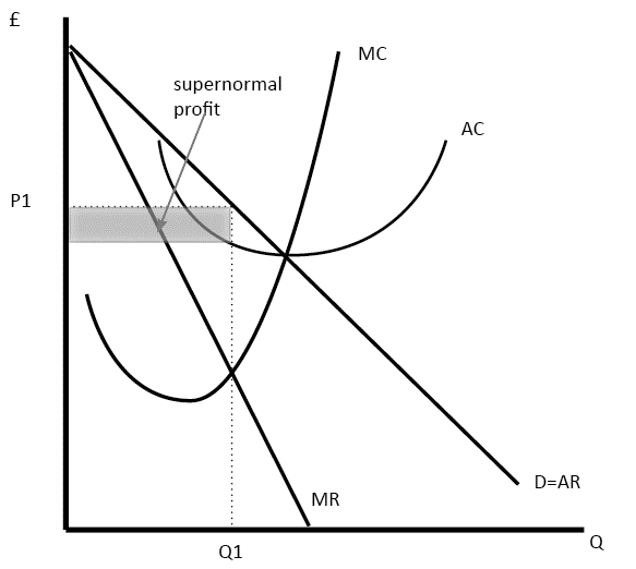
Short-run is the period when at least one factor of production is fixed while the others are variable. The number of entities remains constant in the short run. The firm’s size remains unchanged. The firm’s main objective is to maximize profits (Geroski, 2013). For it to make that happen, it has to continue producing its commodities by maintaining marginal revenue above marginal cost.
From the above diagram, quantity q1 is produced where the MC curve cuts the MR curve. The price is determined by extending q1 until it meets the AR curve. Profit is represented by the grey rectangle and is supernormal (Besanko & Thakor, 2015).
Short-Run Losses in a Monopolistic Competition
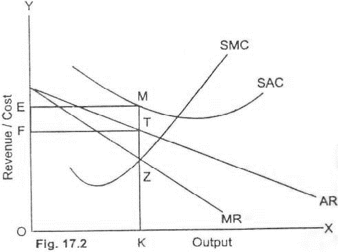
In this case, the AC goes above the market price, and the firm starts incurring losses, which equates to the difference between the AC and the market price multiplied by the output produced. This may make the firm exit the industry if this persists (Helpman & Krugman, 2015).
Long-run equilibrium in a monopolistic competition
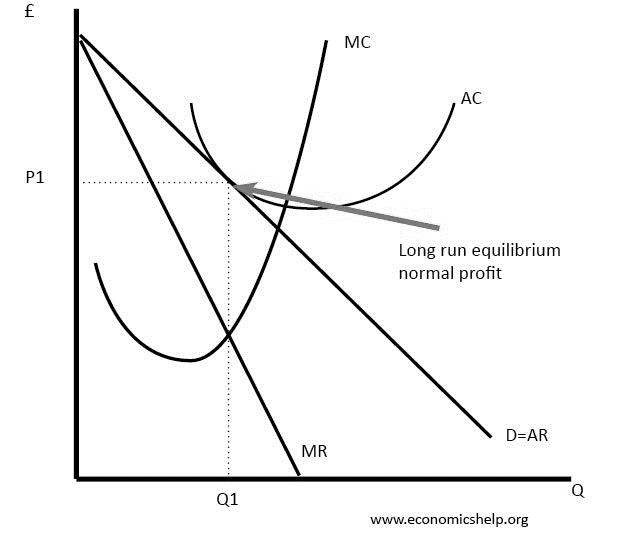
Long-run is the time period when no factors of production are fixed. The firm produces the amount of goods where the long-run marginal cost cuts the marginal revenue. The price, p1, is arrived at by extending q1 until it meets the AR curve (Scherer, 2012).
Oligopolistic Market Structures
An oligopoly is a market structure that is under the control of a few large sellers.
In this type of competition, each player’s actions are influenced by the others and also influence the actions of the others. Each player must consider the actions of the others in their planning. In this type of market structure, there are likely collusions, whereby companies come together with restrictive practices in order to hike prices and control production in a similar way to monopolies (Brander & Lewis, 2013). Such collisions give rise to cartels for the OPEC, which controls oil production internationally.
There exists also what we call price leadership, whereby a firm sets the prices of products, and the others follow. This type of competition employs the game theory in its behaviors.
Characteristics of an Oligopolistic Competition
There are several barriers to entry into the market, such as government licenses, patent rights, economies of scale and the actions of the existing firms.
There are few large firms, and thus, the actions of each firm can influence the actions of the others.
They can make and sustain long-run profits.
Products are homogenous though differentiated.
Each firm has a perfect knowledge of its costs and demand functions, while the consumers have imperfect information about the price, product quality and cost.
There exists non-price competition (Baumol, Contestable markets: an uprising in the theory of industry structure, 2015).
The Kinked Demand Theory under Oligopoly
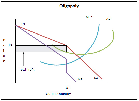
Let us have a look at a situation whereby a firm wants to alter its pricing. The other firms will either go in the same direction or refuse to. If the said firm decides to raise the prices, the other firms will definitely not follow so as to take advantage of the situation and hence increase their market share through their constant pricing (Maskin & Tirole, 2015). The demand curve will, therefore, be more elastic since the customers will prefer buying from the other firms and shy away from the price raiser, thus lowering the revenues of the said actor.
In another scenario, if the firm lowers its prices, the other players will also follow so that they don’t lose their market share. This makes the demand curve to be more inelastic since all of them are acting in unison. This leads to a kink in the demand curve, where the demand changes from very elastic at higher prices to inelastic at lower prices. The MR curve, too, will be kinked as it depends on the prices (Maskin & Tirole, 2015).
The kinked nature of the demand curve elaborates why firms in oligopolies shy away from price changes.
Long-Run Profits in Oligopoly
Firms in this type of market structure can retain long-run abnormal profits. This is due to barriers to entry that exist, thus preventing new entrants who might want to come in and cash on the abnormal profits (Mueller, 2015).
Resource Allocation in Monopolistic Competition
In this kind of rivalry, there are various purchasers and dealers, however numerous organizations are not delivering similar wares. The products of one firm have particular highlights to separate them from those of alternate firms. Because of this item separation, each firm or substance can charge its own value (Baumol and MONTFORT, 2014).
Firms in this sort of rivalry don’t deliver at an ideal scale. It delivers underneath its ideal capability. It implies that the commonness of the overabundance limit comes because of the nearness of misallocation of assets that exists in this sort of rivalry.
This kind of market structure has a tendency to abridge financial proficiency through a few squanders, for example, unused limit, misallocation of assets, item separation and promoting.
Oligopolistic Competition and Resource Allocation
In this sort of rivalry, there exists a misallocation of assets. An oligopoly can appear as a deceitful oligopoly or a non-conniving oligopoly. This could likewise be as a pioneer setting costs and supporters going a similar bearing, generally called value administration.
In all the above kinds of oligopolies, there exist asset misallocations. Taking the instance of a non-tricky oligopoly, we find more noteworthy squandering and misallocation of assets (Brander and Lewis, 2013).
Culminate Competition and Resource Allocation
In this sort of rivalry, advertising costs reflect the finished portion of assets, and furthermore, there is the opportunity for passage and exit. There is ideal information on the market by both the purchasers and the merchants, in spite of the oligopolies and monopolistic rivalries. In this sort of rivalry, no player or gathering of players has the preferred standpoint over the others (Stigler, 2014).
This kind of market structure can be utilized as an ideal measuring stick to stand out from other market structures since it shows elevated amounts of market efficiencies, for example,
Allocative efficiencies whereby, in both the short and long run, costs are equivalent to minor costs (Stigler, 2014). Beneficial efficiencies whereby balance amounts are provided at the most minimal normal expenses.
Case Study of Hindustan Unilever Limited (HUL), a Monopolistic Firm
HUL has the strongest market base in India, which is spread strategically in various market segments under the soaps and detergents market share due to its various brands.
Even with a lot and stiff competition facing it, it has continued to do innovation of new products, hence continuing to dominate the market such that others find it difficult to find their way in.
Contrary to other companies, it has its base under all the market segments enabling it to target a wide range of consumers.
Case Study of Oil Producing and Exporting Countries (OPEC) As an Oligopoly
OPEC was formed by a number of oil-producing nations, especially the Middle East countries, and it operates as an oligopoly. They make the decision of how much oil to pump and the subsequent pricing.
These countries aspire to maintain high prices of oil, but there exist cartels who always attempt to increase production in order to pocket huge shares of total profits. Each time, these countries meet to decide on pricing, but then they do not remain true to their agreements and often cheat (Wilson, 2013).
Oligopolies and Efficiencies
Oligopolies are generally inefficient.
The general rule for efficiency requires that =MC=lowest ATC. Oligopolies contravene this.
Oligopolies tend to sustain economic profits in the long run because they produce at a point where p>minimum average total cost; hence, we can say that they are not productively efficient.
They are neither allocative efficient as they produce where at the point where p>marginal cost.
This is to say that firms in this kind of market structure do not produce in the least costly manner, and they rarely produce the desired amount of goods by society (Wilson, 2013).
At such prices, the quantities produced are often below the quantity at which the lowest ATC is attained. This leads to underallocation of resources.
Monopolistic competition and efficiency
Monopolistic firms do their productions at the point where p>mc. This means that there is under allocation of resources, thus making them allocatively inefficient.
These firms are also productively inefficient as they do not produce at the point where p=lowest ATC, which is a requirement for productive efficiency.
Firms in this market structure operate below optimal capacity due to the presence of excess capacity. A huge presence of product differentiation also gives rise to productive inefficiencies (Wilson, 2013).
Lodging moderateness
This is a term used to allude to the connection between the use of lodging costs, lodging contract installments, lease and family unit receipts.
Lodging Affordability in Australia
Lodging Affordability for Owners
Lodging moderateness has gigantically declined since the late 1970s. In Sydney, where a huge ascent in costs has been seen, discoveries by the Parliamentary Library estimations showed that the proportion of normal dispensable family unit wage to middle house costs had gone up from nearly 3.2 in June 1980 to simply more than 7 in June 2016 (USED, 2015). 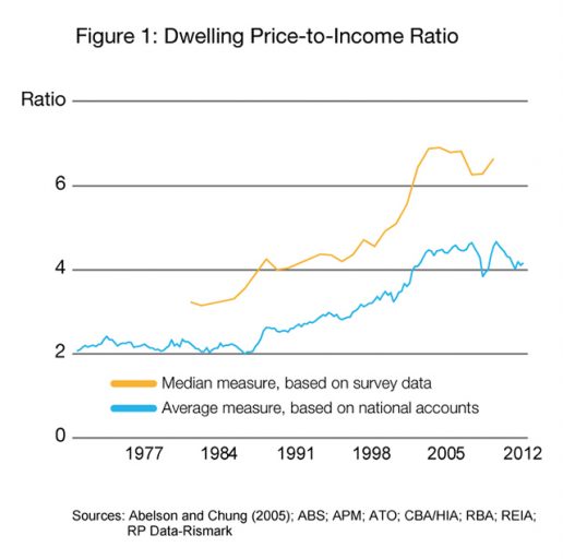 (Brander & Lewis, 2013)
Most of the growth in housing prices in relationship to household incomes occurred during the early 1980s and 2000s. The Reserve Bank of Australia, in 2014, noted that Australian housing prices had increased by about 0.6667% as compared to the relative incomes of the households.
This was attributed partly to the increase in housing prices in the years 1984 and 2010. The Australian Bureau of Statistics indicated that the average weekly household expenditure on the present housing had moved up from 12.8% to 18%. Part of the increase is likely to project the changing societal preferences, whereby households decide to invest more of their household budgets into larger, more luxurious or better-located homes. This has been made possible by the financial deregulation and a robust growth in household disposable incomes between the years 1980-2010.
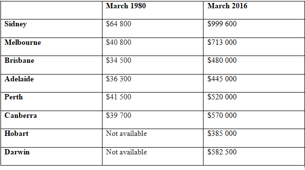
Affordability obviously differs from state to state, territory to territory and also between different capital cities and regional areas.
Capital Cities Nominal Median House Prices  (Kiel & McClain, 2017)
The constant increase in house prices is one of the factors behind the reduction in the levels of home ownership in Australia. Statistics done by the Household, Income and Labor Dynamics in the country revealed that in 2000, 70% of the total households were owner-occupied, as opposed to 65% in the year 2015. Such a trend is mostly evident in Victoria, where we have 7.8%, then New South Wales, where we have 4.3% and then South Australia with 2.5%.
There are two approaches used in determining housing affordability in Australia. The first is the ratio measures, which focuses on interactions between housing expenditure and household receipts (Malpezzi, 2013). Then there is the residual measure which lays emphasis on the capacity of a household to stick to acceptable standards of living after housing expenditures. This method is majorly used by researchers and academicians as it involves a lot of complexity.
Housing Affordability for Renters
The Australian Housing Occupancy and statistics carried out in the year 2014 found that the proportion of the total households who live in rental houses had gone up from 25% to 30%. Added to this were the renters with the private landlords, which had also gone up from the previous 17% to 25% (Wilson, 2013).
The study revealed that generally, the private renters used much of their gross income on housing costs than the tenure types. Going by the study figures, the private renters used approximately 20% of their total income on housing, while 17% were mortgages.
There exists a problem known as ‘housing stress,’ which refers to a situation whereby a household spends more than 30% of its gross income on housing expenditure (USED, 2015).
Government Responses to the Housing Affordability Issue
In January 2016, the government of Australia made it clear that it would form an affordable housing task force. The group was tasked with finding ways of increasing the number of affordable housing for those living on low incomes and subsequent implementation of the same findings (Wilson, 2013).
It came out that if the supply of affordable housing was to realize just enough to counter the medium-term to long-term demands, then a good investment in the affordable end of the residential market has to be made (USED, 2015).
But there is an obstacle to such a plan. It was evident that the institutional investors showed little interest in such affordable housing plans, and this could be hugely attributed to the risks involved, coupled with the low returns in such a pan of erecting affordable housing (USED, 2015).
The government has, in its quest to overcome such investor reluctance, injected some incentives and has also introduced some form of financial instruments to help salvage the situation.
Financial instruments like such could help scale up housing supplies on a long-term basis.
The government has also embarked on a re-arrangement of the tax system designed to control property speculation and price variations (Stigler, 2014).
A Countrywide network of Community Land Trust developments managed by government and housing associations, involving easier transfer of title and improving worker mobility, has also been rolled out.
The government also decided to limit the amount of money that financial institutions can lend to customers (Wilson, 2013).
My Suggestions on the Solutions to the Housing Affordability
Housing affordability problems come up primarily due to the high demand for housing units or due to the high costs that the investors incur during their quest to put up affordable housing. In other words, there is the demand side of the problem and the cost side of it.
Demand Initiated Housing Problems
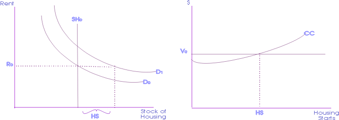
The first diagram shows an increase in demand for housing units. This will definitely push prices up. The increase is shown by D0 to D1. For the prices to remain the same, housing supplies need to be increased from SH0 to HS (Engelhardt, 2015).
The government needs to encourage investment in this particular sector by offering incentives to encourage the players in that field to invest in it (USED, 2015).
(USED, 2015)
Cost-Initiated Housing Problems
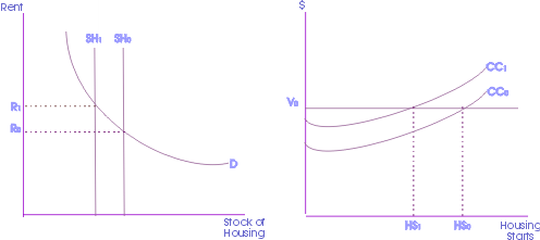
On the below diagrams, if the costs of putting up the housing units increase from CCO to CC1, investors will reduce their house starts from HS0 to HS1. Others will even exit the market. This will make the housing supply reduce from SH1 on the 1st diagram to SH0. Prices will then rise from R0 to R1 (Engelhardt, 2015).
The government once again should come in and offer subsidies so as to lower the costs, an act that shall eventually see more housing being put up to ease the housing affordability issue.
(Engelhardt, 2015)
Cite This Work
To export a reference to this article please select a referencing stye below:
Academic Master Education Team is a group of academic editors and subject specialists responsible for producing structured, research-backed essays across multiple disciplines. Each article is developed following Academic Master’s Editorial Policy and supported by credible academic references. The team ensures clarity, citation accuracy, and adherence to ethical academic writing standards
Content reviewed under Academic Master Editorial Policy.
- This author does not have any more posts.

 (Kiel & McClain, 2017)


