Abstract
Accurate lung cancer classification is essential for efficient treatment scheduling and positive patient outcomes since lung cancer is a prevalent and deadly condition. In this study, offered a cutting-edge method for classifying lung cancer that combines deep learning, feature extraction, and image processing advances. We commence by enhancing lung cancer images through advanced denoising techniques, augmenting the dataset via Generative Adversarial Networks (GANs) to bolster model generalization. Subsequently, we pinpoint the Region of Interest (ROI) employing an Adaptive Correlation Enhanced Active Contour Model (ACE-ACM), followed by extracting rich features utilizing Convolutional Neural Networks (CNNs) based pre-trained models like VGGNet and ResNet. To optimize feature space, we propose a novel hybrid optimization algorithm merging Sea Lion Optimization (SLO) and Sparrow Search Algorithm (SSA), called Sparrow Customized Sealion Optimization (ScLnO), which identifying salient features for focused analysis. The lung cancer classification harnesses the prowess of the DenseEnsembleNet, a sophisticated amalgamation of Optimized DenseNet and CNN, which perform the classification process. Implemented in PYTHON, our framework is poised to revolutionize lung cancer diagnosis, achieved the highest accuracy of 99.19% which is higher than the existing techniques.
Keywords: Lung cancer, Denoising techniques, Generative Adversarial Networks, Region of Interest, Adaptive Correlation Enhanced Active Contour Model and DenseEnsembleNet.
Introduction
One of the most serious and dangerous illnesses in the world is lung cancer. The only way to treat lung cancer is to find it in the early stages. There are several methods that may be used to diagnose lung cancer, such as MRI, isotope, X-ray, and Computer Tomography (CT) [1,2]. PET, CT and X-ray chest radiography, are the three popular anatomic imaging techniques, they are routinely used to identify various lung conditions. CT scans are used by doctors and radiologists to identify and diagnose diseases, instantly see the describe the patterns and severity of illnesses, morphologic extents of diseases, and gauge the clinical progression of diseases and how they react to medicines. Spiral scans, a novel innovation in volumetric CT, irregular breathing cycles, heart motion, and reduce distortions caused by partial volume impacts while significantly accelerating scan durations. As CT technology has evolved, the high-resolution CT test has emerged as the imaging method of choice for the recognition and detection of lung disorders [3, 4, 5]. The task of visually reading or assessing a large number of CT image slices is still difficult despite High-Resolution CT suggesting images of the lung with continually growing anatomic solution.
In contrast to the categorization of benign and malignant [6, 7, 8], the categorization of the three types of lung cancer from medical images is more appropriate to constitute an extremely fine image identification problem due to distinct feature variations and potential malignant characteristics that must be taken into account. The affected region occupies a small percentage of the whole image, rendering the fine-grained characteristics that must be retrieved from images vulnerable to feature noise [9,10]. The vast majority of methods now in use that are based on various deep learning frameworks have demonstrated to have a specific bottleneck in fine-grained scenarios. For the purpose of identifying and categorizing pulmonary diseases, the channel attention mechanism has been employed [11,12]. The presentation of these attentional strategies illustrates the genesis of noise identification from several perspectives. There are several efforts underway to produce computer-assisted methods for diagnosis and detection that will raise the standard of diagnosis for the categorization of lung cancer [13, 14, 15]. Computer-aided systems were created as a result of the need for trustworthy and impartial analyses. To extract characteristics for categorization and severity determination is the goal of this effort.
This research introduces an innovative approach to accurately classify lung cancer, a critical task for effective treatment planning. By combining advanced image processing techniques such as denoising and segmentation with deep learning models like VGGNet and ResNet, intricate features are extracted from lung tumor images. A novel hybrid optimization algorithm further refines feature selection, reducing dimensionality and enhancing focus on crucial aspects. The proposed DenseEnsembleNet, a fusion of optimized DenseNet and CNN, empowers the model to recognize complex patterns. Experimental results on benchmark datasets demonstrate the method’s superiority over traditional approaches, offering promising potential to assist healthcare professionals in early-stage lung cancer diagnosis and treatment decision-making. “The main contribution of the paper is as follows”,
- To effectively extract the lung tumour region, the Adaptive Correlation Enhanced Active Contour Model (ACE-ACM) is used in the medical images using a segmentation algorithm.
- To optimize the feature space and reduce dimensionality, we utilize advanced feature selection algorithm called Sparrow Customized Sealion Optimization (ScLnO), which can include the advantages of both the Sea Lion Optimization (SLO) and Sparrow Search Algorithm (SSA).
- To finetune the hyperparameters of the DenseNet model, the ScLnO algorithm is utilized. The optimized DenseNet model is used along with the CNN for classification of the lung cancer disease.
- To improve the classification process, the Optimized DenseNet and the CNN models are used. The outputs of these two models are concatenated and gives the final classified lung cancer detection output.
The document is constructed in the manner described below, Section 2 included recent publications on lung cancer detection, Sections 3 and 4 provide experimental details, a description of the suggested approach, and a summary of the experiments’ outcomes. In Section 5, the conclusion is mentioned.
Literature review
In this section, the recent existing papers related to the lung cancer detection and their disadvantages are discussed.
In 2022, Kasinathan and Jayakumar [16] have suggested a cloud-based system for the stage-based identification of lung tumours using deep learning. In addition to offering a way for classifying pulmonary illness phases, the study also offers a deep neural network and a cloud-based data collection system for recognizing and validating distinct lung cancer growth stages. The proposed approach offers a hybrid PET/CT imaging methodology called the Cloud based Lung Tumour Analyzer and Stage Classifier. Utilizing industry-accepted benchmark pictures, a multilayer CNN for identifying the various lung cancer types has been designed and validated. The active contour model for lung tumour segmentation was initially built using the recommended Cloud-LTDSC.
In 2021, Sujitha and Seenivasagam [17] have used machine learning and a big data healthcare platform, stage classification of lung cancer. The architecture for the most successful categorization of photos and lung cancer stages was designed in that work using Apache Spark and a streamlining of machine learning techniques. The experiments use threshold technique (T-BMSVM) to categorise tumours into benign and malignant tumours and identify the degree of cancer, respectively. They incorporate binary classification (SVM-nonlinear SVM with Radial Basis Function RBF), multiclass categorization (WTA-SVM winner-takes-all with support vector machine), and multiclass grouping (SVM with winner-takes-all).
In 2020, Asuntha and Srinivasan [18] have introduced a deep learning for the categorization and detection of lung cancer. The scientists found the cancerous lung nodules using cutting-edge Deep learning algorithms. The best feature extraction techniques, such as the Scale Invariant Feature Transform, and Histogram of Oriented Gradients (HoG), Zernike Moment, and Local Binary Pattern, are employed in that study. The Fuzzy Particle Swarm Optimization (FPSO) approach is used to choose the ideal feature following the extraction of textural, geometric, volumetric, and intensity data. The classification of these traits is subsequently done using deep learning. Using a ground-breaking FPSOCNN, CNN’s computational difficulty is reduced.
In 2021, Ibrahim, et. al., [19] have A multi-classification model based on deep learning may be used to identify chest ailments such as COVID-19, pneumonia, and lung cancer. In that paper, it was suggested to use a mix of chest x-ray and CT images to develop a multiple classification deep learning algorithm for the diagnosis of COVID-19, pneumonia, and lung cancer. This combination was chosen because a chest X-ray was less helpful in the early stages of the disease while a chest CT scan was advantageous even before signs occurred and could accurately detect the abnormal characteristics that were seen in pictures. Utilizing these two separate photo types will also increase the dataset and increase classification accuracy. There is currently no deep learning model that can distinguish between these illnesses.
In 2021, Kumar and Bakariya [20] have utilized the deep learning to categorize malignant lung cancer. The author of that research recommends GoogLeNet and Alex Net as deep neural networks. Pretrained CNN was used in experiments on LIDC processing datasets. That work describes an automated technique for identifying lung nodules in areas of interest (ROI). A median filter, Gaussian filter, Gabor filter, and watershed algorithm were added to the DICOM picture size 512 512 to partition the lung sections. (Fully linked) Layers were used by AlexNet, and Pooling Layers were used by GoogleNet.
In 2021, Nanglia, et. al., [21] have suggested a hybrid approach that uses SVM and neural networks to classify lung cancer. The focus of the current study was on the factual information on the potential application of a hybrid Feed-Forward Back Propagation Neural Network for lung cancer deciding. Support Vector Machine (SVM) are used in this situation to develop a hybrid approach that further aids in lowering the computational complexity of the categorization. In light of the previously stated, a three-block system is proposed for categorization, with the first block handling dataset preliminary processing, the following block collecting characteristics using the SURF method, the third block optimizing using an algorithm based on genetics, and the last block executing classification using FFBPNN.
In 2021, Marentakis, et. al., [22] have used the radiomics and deep learning algorithms, lung cancer histology can be determined from CT scans. By using various feature extraction and classification algorithms on pre-treatment CT images, that seek to evaluate the possibility of NSCLC histological categorization into AC and SCC in this study. The used picture dataset (102 patients) came from the TCIA, which was a collection of publicly accessible cancer imaging archives. The suggested method was founded on pretreatment CT imaging, which offers knowledge about the tumor’s geographic heterogeneity as well as its overall picture features. As part of clinical practice prior to therapy, CT imaging does not add any further complication or delay.
In 2022, Shafi, et. al., [23] have used a deep learning-based support vector network, an efficient method for detecting lung cancer from a CT scan. The SVM used in that work, which was deep learning capable, was proposed as a cancer detection model. The physical and pathological modifications in the tissue layers of the cross-section of lung cancer tumours are identified using the advised computer-aided design (CAD) model. The model was originally trained to identify lung cancer by assessments and analyses of the preset profile characteristics in CT scans taken from patients and control patients at the moment of discovery. Using CT pictures of individuals and control subjects who had not participated in the training phase, the model was then evaluated and verified.
In 2023, Pandit, et. al., [24] have recommended the lung cancer categorization deep learning neural network. The suggested technique combines multispacer images in the pooling layer of a CNN utilizing the Adam Algorithm for optimization to increase overall accuracy and diagnose lung cancer. Prior to down sampling via max pooling, the CT images underwent pre-processing by being fed into a convolution filter. An autoencoder model based on a CNN was then used to extract features, and multispacer image reconstruction was employed to decrease error during image reconstruction, improving prediction accuracy for lung nodules. Finally, the SoftMax classifier was used to categorize the CT images using the reconstructed pictures as input.
In 2020, Bicakci, et. al., [25] have suggested the molecular imaging-based sub-classification of lung cancer. Adenocarcinoma (ADC) and squamous cell carcinoma (SqCC), two subtypes of NSCLC, were distinguished in that study using deep learning-based classification algorithms, which were thoroughly studied. The study included PET scans and tumor-containing slices from 94 individuals (88 males), of which 38 had ADC and the remaining had SqCC. To determine how peritumoral regions in PET scans affect the subtype categorization of tumours, three trials were conducted. Each model was optimized using a variety of optimizers and regularization techniques.
2.1. Problem statement
Accurate and prompt detection, classification, and stage prediction are crucial in the research environment surrounding lung cancer diagnosis. The inability of current diagnostic techniques to achieve high levels of accuracy and reliability might result in incorrect diagnoses and delayed actions. The importance of early identification of lung cancer for better patient outcomes highlights the pressing need to create methods for spotting the condition in its early stages. The development of new image processing methods and feature extraction strategies to improve the caliber of medical imaging data, particularly CT scans and PET pictures, is the driving force behind these endeavors. The proper categorization of the various lung cancer stages and subtypes is a difficult task that calls for the creation of strong models that can distinguish between complex disease presentations. Parallel to this, initiatives are being made to reduce deep learning models’ computational complexity while maintaining their diagnostic efficacy. Enhancing diagnosis accuracy may be possible by integrating data from several medical imaging modalities, such as chest X-rays and CT scans. Cloud-based solutions and big data frameworks are being researched to effectively handle the exploding amount of medical imaging data. The use of machine learning and deep learning techniques, which take use of their ability to recognize complex data patterns and draw insightful conclusions, is essential to this endeavor. The ultimate goal is to develop diagnostic models that easily fit into clinical practice, providing medical practitioners with precise and timely information to aid in making knowledgeable decisions. In order to advance the field towards improved lung cancer diagnosis and patient care, this research aims to fill in existing gaps in the literature, such as a thorough model for differentiating between COVID-19, pneumonia, and lung cancer. It also investigates cutting-edge techniques like histology classification and hybrid algorithms.
Proposed methodology
Classifying lung cancer is crucial for medical diagnostics because it has a big influence on patient outcomes and treatment planning. Accurate and effective categorization techniques are essential for the incidence and severity of lung cancer. This section demonstrates accurate categorization and prediction of lung cancer using the technologies enabled by deep learning and image processing. Getting images is the first stage. Additional preprocessing of the images is done using wavelet and NLM denoising. An improvement in visual quality is the outcome. Then used the GANs for data augmentation to further enrich the dataset and increase model generalization. The modified Active Contour Models are then used to segment the pictures. The determination of the region of interest is made easier by this stage. Then, classification techniques based on deep learning are used. Figure 1 displays the block diagram for the suggested lung cancer detection methodology.
Figure 1: Block design of the proposed lung cancer detection system
3.1. Preprocessing
The lung cancer images are preprocessed to enhance image quality and remove any artifacts or noise that may affect the texture analysis. To improve the clarity of images of lung cancer and lower noise, employ advanced denoising techniques such as NLM denoising and wavelet denoising. These methods effectively preserve image details and improve the accuracy of subsequent analysis.
3.1.1. NLM denoising
The NLM noise reduction method was created to eliminate just the noise while minimizing the loss of the image’s fundamental information. After placing regions with the same size mask all around the Region of Interest (ROI), this approach compares the similarities of the intensity and edge information in an image. Additionally, the given weight utilized during image processing increases with the degree of similarity. The NLM method’s fundamental equation is represented as
(1)
Where is the intensity of the noise portion of the nth pixel, is the area around the pixel, is a function based on the weighted similarity (sum of the difference among the desired pixel and its neighbouring pixels), is the normalization constant, and is the Euclidean distance.
3.1.2. Wavelet denoising
Lung cancer detection findings are typically accompanied by a more interference data. Wavelet denoising is a popular technique of time series denoising, hence this technology will be used to train more accurate prediction models. The three steps of wavelet denoising are outlined as follows in accordance with the wavelet denoising approach.
(1) Decomposition: Identify the wavelet basis function and the N decomposition layers. The resulting decomposition of the noisy data into approximation and detail coefficients.
(2) Threshold processing: Choose a threshold function, then calculate each layer’s components.
(3) Reconstruction: By using the modified coefficients, reassemble the data.
The soft threshold and hard threshold parameters of the threshold function are defined in Eq. (2) and Eq. (3), respectively.
(2)
(3)
Where is the wavelet coefficient and denotes the threshold. The data will cause extra oscillation, and the hard threshold function will maintain the signal’s peak characteristics. The wavelet coefficients do, however, maintain a higher level of overall continuity when using the soft threshold function, and the original signal’s smoothness is also preserved. Consequently, the wavelet denoising approach uses a soft threshold function.
- Image Augmentation using GAN model
To further enhance the dataset and improve model generalization, we employ GANs for data augmentation. GANs generate synthetic images that closely resemble real lung cancer images, diversifying the dataset and improving the categorization model’s reliability. The ability of GANs to recognize and comprehend patterns in the training data allows them to produce new data with comparable characteristics. A GAN trained on the collection of images, is able to produce new images that seem realistic to a human observer. The GAN has a generator network and a discriminator network. The discriminator is given the capacity to discriminate between real samples and synthetic samples. Their function of min-max is represented by Eq. (4) and uses the value function
(4)
Where is the genuine data sample taken from , G and D are the generator and discriminator, and is the random (noise) input taken from . The discriminator loss function ( is a typical crossentropy loss function, similar to the binary classifier given in Eq. (5):
(5)
The results of the loss function were very heterogeneous depending on the sorts of input samples employed. The numbers displays the likelihood of properly forecasting the precise and big models, even if f denotes the initial digit.
The loss function of the generator ( seeks to produce as many random variables as possible in order to maximize the loss function of the discriminator (. The loss function of generator is expressed as The breakdown of generator loss is shown in Eq. (6),
( (6)
While training, only one model’s parameters are changed, not those of the second. The generator functions most effectively when the discriminator becomes perplexed and is unable to distinguish between true samples and fake ones. After training, the discriminator is changed until it functions best for the current generator.
- ROI Extraction using ACE-ACM
The lung tumor regions are identified and segmented from the medical images using a segmentation algorithm. This step ensures that the subsequent texture analysis focuses specifically on the relevant regions. In this research work, the ACE-ACM will be applied, to isolate the ROI region from the rest. An effective technique for object recognition and shape analysis is contour. The steps involved in the ACE-ACM is given below,
Step 1: Compute the weight function
The weight function of the pre-processed image is calculated using the adaptive weight function. The mathematical expression of the weight function is given in Eq. (7) as,
(7)
Where denotes the weight function, which is represented by,
(8)
Where represents the base weight of the pre-processed image, and denotes the weight factor that increases the gradient magnitude .
Step 2: Compute the cross correlation-based entropy
After finding the weight function , the cross correlation-based entropy () is calculated using the Eq. (9) below,
(9)
Where represents the template function that represent the expected appearance, denotes the image region around contour point s.
Step 3: Modified energy function computation
The energy function is calculated based on the contour value and the and cross correlation-based entropy value. Which can be defined in Eq. (10) as,
(10)
(11)
- Feature Extraction
From the segmented pictures, useful characteristics should be extracted by employ an advanced feature extraction methods. Instead of relying solely on traditional approaches, we integrate deep learning-based feature extraction models such as pre-trained models like VGGNet and ResNet. These models automatically learn and extract high-level features from lung cancer images, capturing intricate patterns and improving classification accuracy.
- VGG 16
The ImageNet dataset was utilised to pre-train the VGG16 deep neural network, which is used to extract constraint characteristics. The VGG16 architecture comprises of three fully linked layers after the initial five blocks of convolutional layers. In order to maintain identical spatial dimensions as the layer preceding it, each activation map in a convolutional layer uses a 33 kernel with a stride of 1 and padding of 1. With the help of the imported convolutional layer’s parameters, the bottleneck characteristics are retrieved. Each convolution is followed by a ReLU activation, a spatial dimension lowering using the max pooling method. Max pooling layers employ 22 kernels with a stride of 2 and no padding to make sure every spatial dimension of the activation map of the preceding layer is divided in half. After two completely linked layers with 4,096 ReLU activation units, the last 1,000 fully connected softmax layers are used. The VGG16 model has some downsides, including a high evaluation cost and a high memory and parameter need. VGG16 is then made up of 138 million or more parameters. The fully-connected layers include 123 million occurrences of these traits.
- ResNet
ResNet can perform well in a variety of applications, including speech recognition, natural language processing, picture classification, image production, visual identification, and user prediction. Following two weight layers, the input value x’s residual mapping is denoted by and the fundamental mapping is denoted by , respectively. The residual unit converts the issue from matching the connection between to fitting the connection between by employing a function of identity as a short cut link. Two different benefits of the residual network over the standard CNN are discussed below.
- Easier to be optimized
ReLU activation function, which is the activation function before the output layer of the residual unit, frequently acts as an intrinsic value of 0 or an identity function. For learning, we combined many leftover units. If one assumes that the identity functions that activate the ReLU are
(12)
Where stands for the weights and stands for the resnet unit’s input. A direct forward propagated output () and the residual mapping of the resnet unit that has to be learnt are represented by . Following that definition, the residual network’s forward propagation mechanism is
(13)
Where is the total output of the connected residual units of length . On the other hand, a typical CNN’s forward propagation procedure may be characterized as
(14)
In the formula where Wi denotes the weights, and stand for the input and output of the lth and convolutional layers, respectively. Eq. (13) and Eq. (14) may be compared to show that the residual network requires less computing power and can be optimized more easily than the conventional CNN.
- A more effective approach to the gradient issue
According to Eq. (13), the backpropagation procedure may be used to represent the gradient of the residual network as
(15)
Where stands for the model’s loss function. The gradient of a standard CNN may be determined by,
(16)
The traditional CNN is prone to gradient disappearance and explosion issues as the network gets deeper, while the ResNet may successfully address these issues, according to the comparison between Eq. (15) and (16).
- Feature selection using ScLnO
To optimize the feature space and reduce dimensionality, we utilize advanced feature selection algorithm called ScLnO algorithm. The proposed ScLnO algorithm is the combination of the SLO and SSA, respectively. These techniques intelligently identify the most relevant and discriminative features, ensuring that the classification model focuses on the most informative aspects of lung cancer images. The various kinds of sparrows are often social birds. The producer and scrounger are the two separate species of house sparrows that are kept as pets. While the scroungers rely on the producers to provide them with food, the producers actively seek for sources of food. In the meantime, the predatory birds in the flock employ the partners with high intakes as competition for their food sources to increase their individual predation level. The behaviour of the sea Lion is hybrid with the sparrow, to improve the strategies of the sparrow.
Step 1: Initialization
To find food in the simulation experiment, we must utilize computer-generated sparrows. The following matrix can be used to show where sparrows are located:
(17)
where is the total amount of sparrows and represents the dimension of the parameters which have to be optimized.
Step 2: Fitness computation
The fitness of the optimization is computed using the accuracy value. The mathematical expression for the fitness is given in Eq. (18),
(18)
Consequently, the following vector may be used to represent the fitness value for all sparrows:
(19)
This shows the individual’s level of fitness as measured by the length of each row in FX, while n here stands for the number of sparrows. When searching for food in the SSA, producers with higher fitness ratings are given preference. Furthermore, the producers are assumed to be the first 10% of the fitness solutions since they are in charge of directing the scroungers and seeking for food. The other 40% of the fitness solution are classified as scroungers since they follow the producers’ lead and create the majority of the population’s food. In contrast to scroungers, producers have a greater range of options regarding where to seek for food.
Step 3: Sealion based Detection & tracking of prey by scroungers
Using a uniform random distribution in the search space, SLO first creates N (the population’s size) D-dimensional solutions as shown below. Then, in the producers, they locate the prey and attract other members to form the subgroup before organizing the net in accordance with the encircling process. The best current option—or the solution that comes closest to becoming the best solution—is regarded as the prey. Eq. (20) presents these behaviours.
(20)
Where . represents the minimum value of the solution with dimension, similarly is the maximum value of the solution with dimension, is the encircling factor that can controls the step size of the movement. Then the parameter represents the promising area.
Step 4: Producer-Scrounger interaction based on vocalization
A Producer will summon other Scroungers in its group to come together and construct a net to catch the prey when it spots a gathering of its prey. The Producer is regarded as the group’s leader and will direct the Scrounger group’s actions and determine its behaviour. The producers’ instructions serve as the basis for the Scroungers’ positional adjustments. These behaviours are represented mathematically in Eq. (21),
(21)
Where, is the guidance factor, represents the position of the scrounger, denotes the position of the producers. The values of are given in Eq. (22), and Eq. (23), respectively.
(22)
(23)
Where, is the angle of voice refection, is the angle of voice refraction. In our research, is a randomly generated number between [0, 1], and = and
Step 5: Attacking phase (Circling updating position based on tent chaotic map)
Producer hunts the bait ball of prey by starting at the boundaries and pursuing it. Based on a tent-like chaotic map, the position of the circling is updated. The fundamental solution, the current optimal solution, is used to create the tent chaotic sequence. The ideal solution in the series is then utilized to update the position of the food supply, forcing it to depart from the local optimal. In Eq. (24), the mathematical expression is represented as,
(24)
Where, is the tent chaotic map, is the best solution and is the global best solution.
Step 6: Position update of the Scrounger
Certain scroungers pay more attention to the producers. They leave their present place as soon as they learn that the producer has discovered excellent food and begin fighting for it. They can rapidly obtain the food created if they are successful; if not, the laws are still followed. The method for changing the location of the scrounger is provided in Eq. (25) below:
(25)
Where denotes the producer’s ideal position. designates the world’s worst location at the moment. Each member in the 1 d matrix is given a random number between 1 and 1, and = . The scrounger with the lowest fitness grade has a higher chance of going hungry when .
Step 7: Save the so far acquired best solution.
Step 8: Return the best solution
Step 9: Terminate the condition
| Algorithm 1: Pseudocode for ScLnO algorithm |
| Step 1: Initialization X[N][m] = Initialize Sparrows Position Matrix () // Eq. (17) Step 2: Fitness Computation F_X[N][m] = Calculate Fitness Matrix(X) // Eq. (18), Eq. (19) Step 3: Detection & Tracking of Prey by Scroungers Initialize Solutions(X) // Eq. (20) Step 4: Producer-Scrounger Interaction based on Vocalization Update Scrounger Positions(X) // Eq. (21) Step 5: Attacking Phase (Updating Position based on Tent Chaotic Map) Update Producer Positions(X) // Eq. (24) Step 6: Position Update of the Scrounger Update Scrounger Positions Based On Conditions(X) // Eq. (25) Step 7: Save the Best Solution So Far Save Best Solution(X) Step 8: Return the Best Solution Return Best Solution(X) Step 9: Terminate Condition if Termination Condition Met () then Terminate Simulation () |
After performing the feature selection task, the selected optimal features are given to the DenseEnsembleNet classifier for classifying the lung cancer disease image. For this classification purpose, the hyper parameters of the DenseNet model is fine tuned using the ScLnO algorithm.
- Lung cancer classification using DenseEnsembleNet
This DenseEnsembleNet is the combination of the optimized DenseNet and CNN. DenseNet models facilitate feature reuse and gradient flow, enabling effective learning and representation of complex patterns in lung cancer images. We fine-tune the DenseNet model using advanced optimization algorithms, which optimize the network’s weights and improve the overall classification performance. The architecture of the DenseEnsembleNet is shown in figure 2.
Figure 2: Layered architecture of the DenseEnsembleNet
- DenseNet
The DenseNet consists of transition layers, dense layers (completely linked layers), max pool layers, and convolutional layers. The architecture of the model is activated with ReLU throughout, and the top layer is activated with SoftMax. The convolutional layers restore the properties of the picture while the maxpool layers lower the dimensionality of the input. The fully connected layers come after the initial flattened layer in the stack. One input array is sent to the flatten layer, which performs as an artificial neural network. The hyperparameters of the DenseNet model is fine tunes using the ScLnO algorithm.
- Convolution Layer
In simple terms, a convolutional layer augments an input with a filter, resulting in the activation. A feature map that displays the intensity of the found features at various positions within the input is the result of constantly applying the filter to an input. A feature map that has been produced using a number of filters can then be subjected to activation processes like ReLU. Since the filter used in a convolutional layer is narrower than the input data, the operation performed among these two entities is frequently a dot product. The result of this layer would be , supposing a square neuron element, and a filter having a size of follow. According to Eq. (26), the inputs from the layer cells before them must be summed up in order to determine the nonlinear input to the unit .
(26)
Eq. (27) illustrates how the convolutional layer implements the determined non-linearity.
(27)
- MaxPool Layer
Reducing the dimensionality of the characteristic map is the primary goal of including a maxpool layer into a CNN. The maxpool layer applies a filter to the feature map in a manner similar to the previous layer, summarizing the features in the area that the pooling layer has filtered. The following dimensions are presumable to be present in a feature map: , which stand for the feature map’s height, width, and channels, respectively. When the maximum pooling () across the size f and stride s filters is used, Eq. (28) determines the dimensions of the feature map.
(28)
- Transition Layer
In order to simplify the model, a CNN employs a transition layer. Typically, a transition layer will make use of a stride 2 filter to halve the input’s height and width and an 11 layer of convolution to reduce the total of channels.
- SoftMax Activation layer
The softmax activation function is frequently used in deep learning systems to solve classification problems. The general structure of a nonlinear activation function is defined by Eq. (29), where weight is denoted by the variable and bias is denoted by the variable b over an input vector .
(29)
When estimating the probability of each output class, a convolutional neural network’s output layer uses the softmax function. Every neuron in the output layer receives one value as per the specification of the softmax function. The possibility (or probability) of a certain node reaching the output by each of these neurons in the output layer. The softmax function is defined over the softmax function , applied to the input concerns the exponential function of the input vector denoted by and the exponent function of the output vector denoted by with m instances as stated in Eq. (30)
(30)
The binary cross-entropy loss function and softmax were used in this work as the loss function and activation function, respectively. Binarization problems have been addressed in the past using binary cross-entropy. For a network with n layers, the binary cross-entropy loss function is shown in Eq. (31) and Eq. (32).
(31)
(32)
Where the variable stands for output class for output class 0, reflects the likelihood of the output class 1 and (1-) for the result associated with class 0.
- Dense layer
Most classification at the network’s end takes place in the fully connected layer. In contrast to pooling and convolution, it is a worldwide process. Using data from the feature extraction stages, the output of all the previous layers is submitted to a global analysis. In doing so, it generates a non-linear mixture of the traits that are used to categorize data.
A neural network is said to be tightly coupled when every neuron in a thick layer communicates with every neuron in the layer above it. Whenever each neuron in this layer transmits information to its corresponding neuron in the layer below, a matrix-vector multiplication takes place. Given in Eq. (29) is the formula for matrix-vector multiplication.
(33)
According to the equation above, the variables each represent matrices with dimensions of and , respectively. During training, backpropagation may be used to update the parameters of the preceding layer, which make up the variable matrix. Eq. (34) and Eq. (35) are used to backpropagate over the learning rate that is defined by to change the weights for the layer identified by and bias indicated by the variable of the neural network.
(34)
(35)
A chain rule is used to compute the and (from the output layer via the hidden layers to the input layer). These are the loss function’s partial derivatives of and b are and . Eq. (36)– Eq. (39) are used to compute and .
(36)
(37)
(38)
(39)
According to the aforementioned equations, the variable is the layer linear activation, and is the differential of the -related non-linear function. The nonlinear activation function at the same layer is denoted by .
- Fully connected layer
The fully connected layer mixes the learnt features from various regions of the input picture and conducts feature aggregation. This aggregation allows the network to capture higher-level patterns and relationships between features, leading to more complex representations. In this task, the fully connected layer’s output is often used to make final predictions, the burst assemble is performed. The final FC consist of two layers, this is the final layer of the DenseEnsembleNet model, which give the final lung cancer prediction output. The image flow of the input images at each stage is shown in figure 3.
Figure 3: Input image at each stage
Figure 3 provides illustrative examples showcasing the sequential analysis of two distinct sample images, each representing a specific scenario in lung cancer detection. The first image in the sequence corresponds to a healthy lung, while the second image portrays a lung affected by cancerous growth. Each of these images undergoes a step-by-step process to elucidate the identification process in a comprehensive manner.
- Result and discussion
In this section, the results obtained for the proposed method is compared with the existing techniques. In this work there is two types of datasets are used. Dataset 1 is used for predict whether the lung cancer is present or not, and the dataset 2 is used for find the type of the lung cancer. The detailed description of the two datasets are given below.
- Dataset 1
The IQ-OTH/NCCD lung cancer dataset [26] is taken as the input image and the PYTHON plat form is employed for implementation. The IQ-OTH/NCCD lung cancer dataset, which includes CT scans from both lung cancer patients and healthy participants, was gathered from specialized hospitals over the course of three months in 2019. The dataset consists of 1190 CT scan slices from 110 instances that have been classified as benign, malignant, or normal by medical professionals. Siemens SOMATOM scanners were used to acquire the scans, and a precise CT procedure was followed. Implementation of privacy safeguards was approved by the institutional review board. Each case includes many chest slices, and the dataset represents the variety of occupations and demographics in Iraq, offering a thorough resource for lung cancer research. The total data is divided into two categories called, training and testing. For training, there is 70% of data is used and for testing the remaining 30% of data is used. The performance metrics are used for evaluation.
- Dataset 2
The second dataset is Chest CT-Scan images Dataset [27]. For training, there is 70% of data is used, for testing 20% of the data is used and the remaining 10% of data is used The dataset for the chest cancer detection project consists of medical images in JPG or PNG format, rather than the DICOM format, to align with the requirements of the machine learning model. It encompasses images related to three distinct chest cancer types, namely Adenocarcinoma, Large cell carcinoma, and Squamous cell carcinoma. Additionally, there is a folder containing images representing normal chest cells. The dataset has been meticulously collected and cleaned from various sources, ensuring its suitability for training and evaluating the CNN-based model designed for chest cancer classification and diagnosis.
4.1. Performance metrics
The performance metrics and their calculation formulas are given below.
- Sensitivity
To determine the sensitivity value, just divide the total positives by the percentage of genuine positive predictions.
(40)
- Specificity
The specificity of a prediction is evaluated by exactly dividing the number of projected negative outcomes by the total number of negatives.
(41)
- Accuracy
The accuracy is computed as the proportion of correctly sorted data to all other data in the stream. The level of accuracy is defined as,
(42)
- Precision
It is the depiction of the complete number of authentic values that are properly taken into account throughout the classification process by using the full number of samples utilized in the classification procedure.
(43)
- Recall
Estimating the quantity of genuine samples used in data classification when utilizing all samples from the same categories from the training data is known as the recall rate.
(44)
- F- Measure
The definition of the F-score is the harmonic mean of recall rate and accuracy.
(45)
- Negative Prediction Value (NPV)
NPV describes the effectiveness of a diagnostic test or similar quantitative metric.
(46)
- Matthews correlation coefficient (MCC)
The two-by-two binary factor correlation measurement, sometimes referred to as MCC, is shown in the equation below,
(47)
- False Positive Ratio (FPR)
The number of negative instances divided by the total amount of negative occurrences that are mistakenly broken down into positive yields.
(48)
- False Negative Ratio (FNR)
The likelihood that a real positive may not be picked up by the test is represented by the false-negative rate, sometimes referred to as the “miss rate”.
(49)
- Overall comparison of the proposed lung cancer detection model
The proposed lung cancer detection model (ScLnO + DenseEnsembleNet) is compared with the existing techniques like CNN [16], SVM [23], SLO, SSA and the proposed DenseEnsembleNet classifier (Pro-classifier). The comparison is shown in table 1.
Table 1: Overall comparison of the proposed lung cancer detection model (Dataset 1)
| Metrics | CNN [16] | SVM [23] | DenseEnsembleNet | SLO | SSA | Proposed |
| Accuracy | 0.9798 | 0.8563 | 0.9859 | 0.9455 | 0.9232 | 0.9919 |
| Precision | 0.9697 | 0.8486 | 0.9788 | 0.9182 | 0.8848 | 0.9879 |
| Sensitivity | 0.9697 | 0.8236 | 0.9788 | 0.9182 | 0.8848 | 0.9879 |
| Specificity | 0.9848 | 0.8264 | 0.9894 | 0.9591 | 0.9424 | 0.9939 |
| F-Measure | 0.9697 | 0.8236 | 0.9788 | 0.9182 | 0.8848 | 0.9879 |
| MCC | 0.9545 | 0.8123 | 0.9682 | 0.8773 | 0.8273 | 0.9818 |
| NPV | 0.9848 | 0.8096 | 0.9894 | 0.9591 | 0.9424 | 0.9939 |
| FPR | 0.0152 | 0.0623 | 0.0106 | 0.0409 | 0.0576 | 0.0061 |
| FNR | 0.0303 | 0.0921 | 0.0212 | 0.0818 | 0.1152 | 0.0121 |
The table provides a thorough analysis of several categorization methods utilizing a number of metrics. With a 97.98% accuracy rate, the “CNN [16]” model performs admirably, accurately classifying the bulk of occurrences. It exhibits respectable specificity (98.48%), balanced accuracy (96.97%), and sensitivity (96.97%). With an accuracy of 98.59%, high precision (97.88%), high sensitivity (97.88%), and remarkable specificity (98.94%), the “HSLSO” approach shines. The “PROPOSED” model excels with exceptional accuracy of 99.19%, sensitivity of 98.79%, amazing precision of 98.79%, and specificity of 99.39%, making it the top performer. The “SVM [23]” model, on the other hand, receives scores that are significantly lower, with an accuracy of 85.63% and comparable reductions in precision (84.86%) and sensitivity (82.36%). The accuracy values for the “SLO” and “SSA” approaches are 94.55% and 92.32%, respectively, demonstrating moderate to good performance across a range of measures. In the end, the selection of the best appropriate model would rely on the unique requirements of the classification assignment, whether those criteria were obtaining remarkable overall accuracy and specificity or striking a compromise between precision and sensitivity.
Table 2: Overall comparison of the proposed lung cancer classification model (Dataset 2)
| Performance metrics | CNN [16] | SVM [23] | DenseEnsembleNet | SLO | SSA | Proposed |
| accuracy | 0.9778 | 0.8505 | 0.9859 | 0.9556 | 0.9131 | 0.9960 |
| precision | 0.9667 | 0.7758 | 0.9788 | 0.9333 | 0.8697 | 0.9939 |
| sensitivity | 0.9667 | 0.7758 | 0.9788 | 0.9333 | 0.8697 | 0.9939 |
| specificity | 0.9833 | 0.8879 | 0.9894 | 0.9667 | 0.9348 | 0.9970 |
| F-measure | 0.9667 | 0.7758 | 0.9788 | 0.9333 | 0.8697 | 0.9939 |
| MCC | 0.9500 | 0.6636 | 0.9682 | 0.9000 | 0.8045 | 0.9909 |
| NPV | 0.9833 | 0.8879 | 0.9894 | 0.9667 | 0.9348 | 0.9970 |
| FPR | 0.0167 | 0.1121 | 0.0106 | 0.0333 | 0.0652 | 0.0030 |
| FNR | 0.0333 | 0.2242 | 0.0212 | 0.0667 | 0.1303 | 0.0061 |
The table displays performance metrics for different classification models, including CNN, SVM, DenseEnsembleNet, SLO, SSA, and “proposed”, evaluating their effectiveness in binary classification tasks. CNN achieved 97.78% accuracy, while “proposed” exhibited remarkable precision at 0.9939 and high sensitivity at 0.9939. The “proposed” also demonstrated strong specificity at 0.9970, low FPR at 0.0030, and reduced false negatives (FNR) at 0.0061. These metrics collectively assess the models’ suitability for specific applications like disease diagnosis.
- Accuracy
The accuracy values in the table represent the proportion of correctly classified instances for each model. Figure 4 compares the accuracy metrics for the proposed and current approaches.
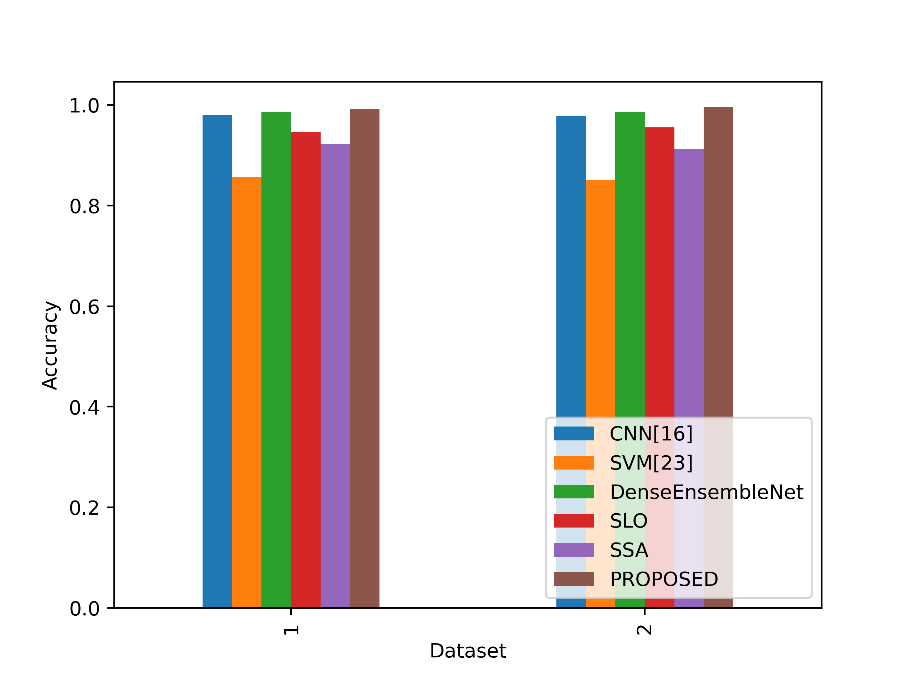
Figure 4: Comparison of the accuracy metrics for dataset 1 and 2
In Table 1, the proposed lung cancer detection model (PROPOSED) achieves the highest accuracy of 99.19% in Dataset 1, indicating its exceptional ability to correctly classify cases. In Table 2, the “proposed” model outperforms other models with an accuracy of 99.60% in Dataset 2, demonstrating its superior performance in lung cancer classification. These accuracy values reflect the proportion of correctly identified cases and highlight the strong capabilities of these models in their respective datasets for detecting and classifying lung cancer.
- Precision
The precision values in the table reflect the accuracy of positive predictions made by each model. In Figure 5, the accuracy values for the suggested and existing approaches are contrasted.
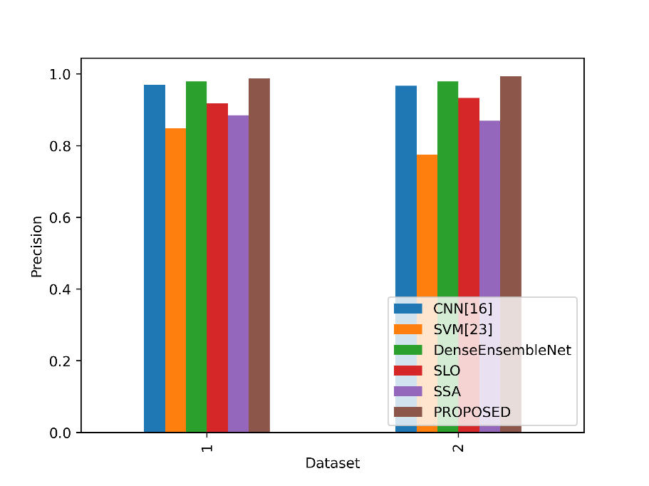
Figure 5: Comparison of the precision values
In Table 1, the “PROPOSED” model achieves the highest precision of 98.79%, signifying that it correctly identifies lung cancer cases with great accuracy. In Table 2, the “proposed” model also excels with a precision of 99.39%, indicating its precision in classifying lung cancer cases. Higher precision values mean fewer false-positive predictions, making models with high precision more reliable in accurately identifying positive cases of lung cancer in their respective datasets.
- Sensitivity
Sensitivity values in the table represent the model’s ability to correctly identify actual positive instances. In figure 6, the sensitivity values of the proposed and existing strategies are compared.
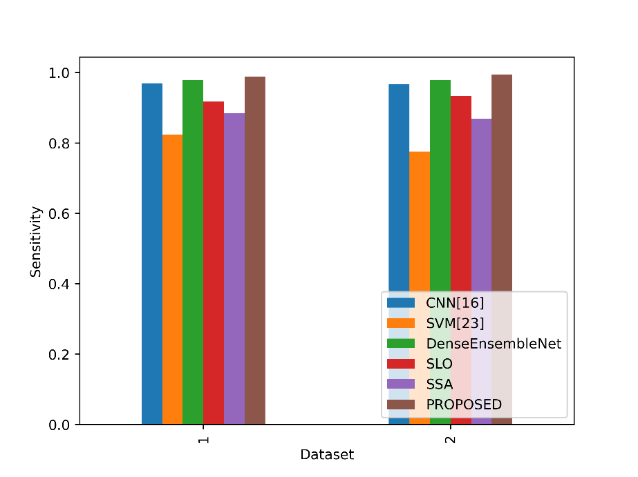
Figure 6: Comparison of the sensitivity metrics
In both datasets, the sensitivity values measure the ability of models to correctly identify positive cases (lung cancer cases). In Dataset 1, the Proposed model achieves a sensitivity of 0.9879, which is higher than the sensitivity of all other models listed. In Dataset 2, the Proposed model again outperforms the other models with a sensitivity of 0.9939, demonstrating its superior ability to correctly detect lung cancer cases in both datasets. This indicates that the Proposed model is particularly effective at identifying positive cases, making it a promising choice for lung cancer detection and classification tasks.
- Specificity
Specificity values in the table reflect the model’s ability to correctly identify actual negative instances. Figure 7 contrasts the specificity ratings for the proposed and current strategies.
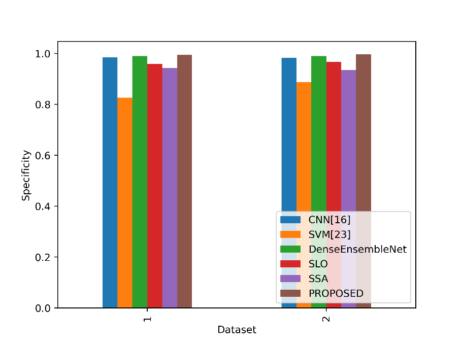
Figure 7: Sensitivity metrics comparison
The specificity ratings in Datasets 1 and 2 assess how well models can recognise negative instances (cases without lung cancer). The Proposed model outperforms all other models in Dataset 1 in terms of specificity, achieving a value of 0.9939. With a specificity of 0.9970 in Dataset 2, the Proposed model performs better than the competing models and demonstrates its greater capacity to identify non-lung cancer patients. This shows that the Proposed model is a strong option for differentiating non-lung cancer patients in both datasets since it performs exceptionally well in detecting negative instances.
- F-Measure
A balanced evaluation of a model’s performance that takes into account both factors is provided by the F-Measure values in the table, which indicate the harmonic mean of accuracy and sensitivity. Figure 8 contrasts the F-Measure values for the suggested and current methods.
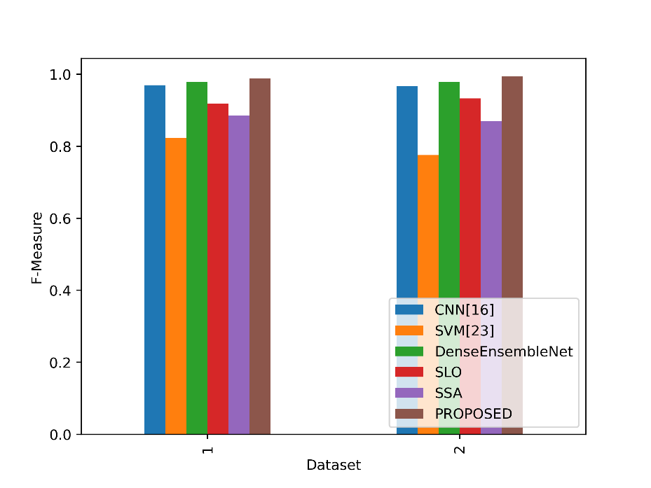
Figure 8: Comparison of the F-Measure metrics
The Proposed model outperforms all other models in both Dataset 1 and Dataset 2 in terms of F-Measure values. The proposed model’s F-Measure in Dataset 1 is 0.9879, which indicates that accuracy and sensitivity are well-balanced. The Proposed model performs much better in Dataset 2, with an F-Measure of 0.9939 indicating a great capacity to balance sensitivity and accuracy. This implies that the proposed model is capable of reaching high accuracy and sensitivity, giving it a trustworthy option for lung cancer detection and classification tasks in both datasets.
- MCC
Based on true positive, true negative, false positive, and false negative outcomes, the MCC values in the table serve as a gauge of how well a binary classification model predicts. Figure 9 shows a comparison of the MCC values for the proposed and existing methodologies.
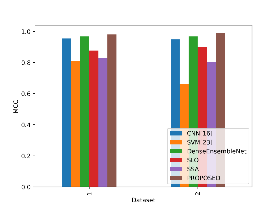
Figure 9: Comparison of the MCC values
The Proposed model obtains the greatest MCC values of all the stated models in both Datasets 1 and 2. The proposed model performed exceptionally well overall in categorising lung cancer cases and non-lung cancer cases in Dataset 1, with an MCC of 0.9818. The Proposed model performs even better in Dataset 2, with an even higher MCC of 0.9909, indicating its reliability in handling the classification job while taking into account both positive and negative instances equally. This implies that the Proposed model is an excellent option for lung cancer detection and classification, offering a thorough analysis of its performance in both datasets.
- NPV
NPV in the table indicates the model’s ability to correctly identify true negative instances among the predicted negatives. In figure 10, the NPV values of the proposed and existing strategies are compared.

Figure 10: NPV values comparison
The Proposed model gets the best NPV values across all the models stated in both Dataset 1 and Dataset 2. The proposed model’s NPV in Dataset 1 is 0.9939, which shows that a significant number of events the model predicts as negative are indeed genuine negatives. The Proposed model has an even higher NPV in Dataset 2, 0.9970, indicating a great capacity to properly identify cases of non-lung cancer when they are predicted to be negative. This shows that the proposed model is dependable for reliably categorizing non-lung cancer cases in both datasets, is successful at reducing false negatives, and minimizes false positives.
- FNR
The FNR values in the table show the percentage of positive events that each model misclassified as negatives. Figure 11 contrasts the FNR ratings for the proposed and current strategies.
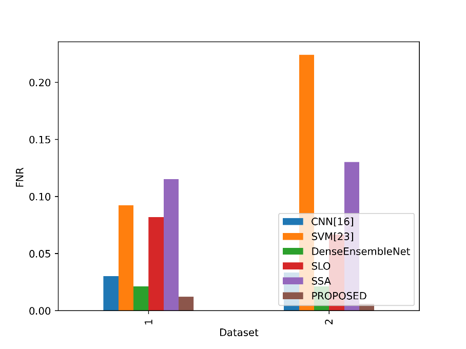
Figure 11: Values of FNR for the Suggested and Existing Methods
The Proposed model obtains the lowest FNR values of all the stated models in both Datasets 1 and 2. The proposed model has an FNR of 0.0121 in Dataset 1, which indicates that it only misses a small number of real lung cancer cases. The Proposed model had an even lower FNR of 0.0061 in Dataset 2, indicating a decreased percentage of missed lung cancer cases. This demonstrates the excellent sensitivity and efficacy of the proposed approach in accurately detecting lung cancer cases and reducing false negatives in both datasets.
- FPR
The FPR numbers in the table show the percentage of real negative events that each model misclassified as positives. A lower FPR means that the model is doing better since it is less likely to mistakenly identify negatives as positives. Figure 12 contrasts the FPR values for the suggested and current methods.
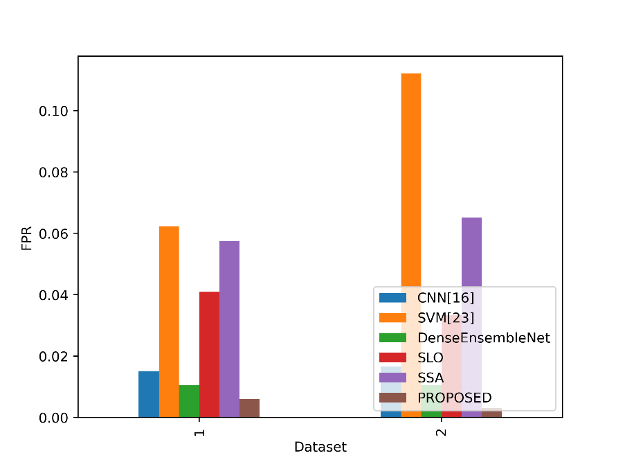
Figure 12: FPR values for the suggested and current methods
The Proposed model obtains the lowest FPR values of all the stated models in both Datasets 1 and 2. The proposed model has a very low rate of false positive predictions for cases other than lung cancer in Dataset 1, with an FPR of 0.0061. The proposed model’s FPR in Dataset 2 is significantly lower, at 0.0030, suggesting a decreased percentage of false positives. This indicates the Proposed model’s excellent specificity and reliability in accurately categorizing non-lung cancer patients and reducing false alarms in both datasets.
Conclusion
In conclusion, the accurate classification of lung cancer holds paramount significance for effective treatment planning and positive patient outcomes due to the gravity of this prevalent and life-threatening ailment. This study has introduced a pioneering methodology that amalgamates cutting-edge advancements in deep learning, feature extraction, and image processing. By capitalizing on advanced denoising techniques and harnessing GANs for dataset augmentation, our approach ensures both enhanced image quality and improved model generalization. The incorporation of the ACE-ACM facilitates precise ROI identification, followed by the extraction of intricate features through VGGNet and ResNet. Our novel hybrid optimization algorithm ScLnO, intelligently identify key features, thus refining the analysis process. The classification stage leverages the potent capabilities of the DenseEnsembleNet, a fusion of the Optimized DenseNet and CNN, resulting in exceptional accuracy. This innovative framework has the potential to revolutionize lung cancer diagnosis, as evidenced by its remarkable accuracy rate of 99.19%, surpassing existing techniques. The integration of cutting-edge technologies has paved the way for a robust and promising solution in lung cancer classification, underscoring the potential for enhanced medical diagnostics and patient care.
Reference
- Braveen, M., Nachiyappan, S., Seetha, R., Anusha, K., Ahilan, A., Prasanth, A. and Jeyam, A., 2023. ALBAE feature extraction based lung pneumonia and cancer classification. Soft Computing, pp.1-14.
- Ukwuoma, C.C., Qin, Z., Heyat, M.B.B., Akhtar, F., Smahi, A., Jackson, J.K., Furqan Qadri, S., Muaad, A.Y., Monday, H.N. and Nneji, G.U., 2022. Automated lung-related pneumonia and COVID-19 detection based on novel feature extraction framework and vision transformer approaches using chest X-ray images. Bioengineering, 9(11), p.709.
- Tielemans, B., Dekoster, K., Verleden, S.E., Sawall, S., Leszczyński, B., Laperre, K., Vanstapel, A., Verschakelen, J., Kachelriess, M., Verbeken, E. and Swoger, J., 2020. From mouse to man and back: closing the correlation gap between imaging and histopathology for lung diseases. Diagnostics, 10(9), p.636.
- Exarchos, K.P., Gkrepi, G., Kostikas, K. and Gogali, A., 2023. Recent Advances of Artificial Intelligence Applications in Interstitial Lung Diseases. Diagnostics, 13(13), p.2303.
- Patel, R.K. and Kashyap, M., 2022. Automated diagnosis of COVID stages from lung CT images using statistical features in 2-dimensional flexible analytic wavelet transform. Biocybernetics and Biomedical Engineering, 42(3), pp.829-841.
- Hage Chehade, A., Abdallah, N., Marion, J.M., Oueidat, M. and Chauvet, P., 2022. Lung and colon cancer classification using medical imaging: A feature engineering approach. Physical and Engineering Sciences in Medicine, 45(3), pp.729-746.
- Saleh, A.Y., Chin, C.K., Penshie, V. and Al-Absi, H.R.H., 2021. Lung cancer medical images classification using hybrid CNN-SVM. International Journal of Advances in Intelligent Informatics, 7(2), pp.151-162.
- Said, Y., Alsheikhy, A.A., Shawly, T. and Lahza, H., 2023. Medical images segmentation for lung cancer diagnosis based on deep learning architectures. Diagnostics, 13(3), p.546.
- Qin, R., Wang, Z., Jiang, L., Qiao, K., Hai, J., Chen, J., Xu, J., Shi, D. and Yan, B., 2020. Fine-grained lung cancer classification from PET and CT images based on multidimensional attention mechanism. Complexity, 2020, pp.1-12.
- Zhao, S., Li, Z., Chen, Y., Zhao, W., Xie, X., Liu, J., Zhao, D. and Li, Y., 2021. SCOAT-Net: A novel network for segmenting COVID-19 lung opacification from CT images. Pattern Recognition, 119, p.108109.
- Wall, C., Zhang, L., Yu, Y., Kumar, A. and Gao, R., 2022. A deep ensemble neural network with attention mechanisms for lung abnormality classification using audio inputs. Sensors, 22(15), p.5566.
- Sun, J., Liao, X., Yan, Y., Zhang, X., Sun, J., Tan, W., Liu, B., Wu, J., Guo, Q., Gao, S. and Li, Z., 2022. Detection and staging of chronic obstructive pulmonary disease using a computed tomography–based weakly supervised deep learning approach. European Radiology, 32(8), pp.5319-5329.
- Shaffie, A., Soliman, A., Eledkawy, A., van Berkel, V. and El-Baz, A., 2022. Computer-assisted image processing system for early assessment of lung nodule malignancy. Cancers, 14(5), p.1117.
- Adams, S.J., Madtes, D.K., Burbridge, B., Johnston, J., Goldberg, I.G., Siegel, E.L., Babyn, P., Nair, V.S. and Calhoun, M.E., 2023. Clinical impact and generalizability of a computer-assisted diagnostic tool to risk-stratify lung nodules with CT. Journal of the American College of Radiology, 20(2), pp.232-242.
- Juan, J., Monsó, E., Lozano, C., Cufí, M., Subías-Beltrán, P., Ruiz-Dern, L., Rafael-Palou, X., Andreu, M., Castañer, E., Gallardo, X. and Ullastres, A., 2023. Computer-assisted diagnosis for an early identification of lung cancer in chest X rays. Scientific Reports, 13(1), p.7720.
- Kasinathan, G. and Jayakumar, S., 2022. Cloud-based lung tumor detection and stage classification using deep learning techniques. BioMed Research International, 2022.
- Sujitha, R. and Seenivasagam, V., 2021. Classification of lung cancer stages with machine learning over big data healthcare framework. Journal of Ambient Intelligence and Humanized Computing, 12, pp.5639-5649.
- Asuntha, A. and Srinivasan, A., 2020. Deep learning for lung Cancer detection and classification. Multimedia Tools and Applications, 79, pp.7731-7762.
- Ibrahim, D.M., Elshennawy, N.M. and Sarhan, A.M., 2021. Deep-chest: Multi-classification deep learning model for diagnosing COVID-19, pneumonia, and lung cancer chest diseases. Computers in biology and medicine, 132, p.104348.
- Kumar, V. and Bakariya, B., 2021. Classification of malignant lung cancer using deep learning. Journal of Medical Engineering & Technology, 45(2), pp.85-93.
- Nanglia, P., Kumar, S., Mahajan, A.N., Singh, P. and Rathee, D., 2021. A hybrid algorithm for lung cancer classification using SVM and Neural Networks. ICT Express, 7(3), pp.335-341.
- Marentakis, P., Karaiskos, P., Kouloulias, V., Kelekis, N., Argentos, S., Oikonomopoulos, N. and Loukas, C., 2021. Lung cancer histology classification from CT images based on radiomics and deep learning models. Medical & Biological Engineering & Computing, 59, pp.215-226.
- Shafi, I., Din, S., Khan, A., Díez, I.D.L.T., Casanova, R.D.J.P., Pifarre, K.T. and Ashraf, I., 2022. An effective method for lung cancer diagnosis from ct scan using deep learning-based support vector network. Cancers, 14(21), p.5457.
- Pandit, B.R., Alsadoon, A., Prasad, P.W.C., Al Aloussi, S., Rashid, T.A., Alsadoon, O.H. and Jerew, O.D., 2023. Deep learning neural network for lung cancer classification: enhanced optimization function. Multimedia Tools and Applications, 82(5), pp.6605-6624.
- Bicakci, M., Ayyildiz, O., Aydin, Z., Basturk, A., Karacavus, S. and Yilmaz, B., 2020. Metabolic imaging based sub-classification of lung cancer. IEEE Access, 8, pp.218470-218476.
- Dataset is taken from www.kaggle.com/datasets/hamdallak/the-iqothnccd-lung-cancer-dataset dated on 07/08/2023.
- Dataset is taken from www.kaggle.com/datasets/hamdallak/the-iqothnccd-lung-cancer-dataset dated on 07/08/2023.
Cite This Work
To export a reference to this article please select a referencing stye below:

Academic Master Education Team is a group of academic editors and subject specialists responsible for producing structured, research-backed essays across multiple disciplines. Each article is developed following Academic Master’s Editorial Policy and supported by credible academic references. The team ensures clarity, citation accuracy, and adherence to ethical academic writing standards
Content reviewed under Academic Master Editorial Policy.