Abstract
Leukemia, a malignant blood cancer, poses a significant health threat, particularly when not diagnosed promptly and accurately. This paper developed a comprehensive approach to leukemia cancer detection leveraging advanced techniques and technology. To enhance the model’s robustness and ability to generalize, a Generative Adversarial Network (GAN) is employed for image augmentation. The progression continues with a sequence of preprocessing procedures. Gaussian Blur is applied to reduce noise and improve image quality, while Histogram Equalization enhances image contrast, facilitating subsequent analyses. An essential element of this framework is a customized Cellular Instance Segmentation (CIS) algorithm for precise cell identification. Following segmentation, an array of features is extracted from these cells, encompassing shape-based, texture-based, and intensity-based descriptors. To optimize the extracted features, a Hybrid Predatory Search Behavior Integration (HPSBI), amalgamating the Beetle Antennae Search (BAS) and Marine Predators Algorithm (MPA), is deployed. The core of this framework is LeukemiaNet model, an amalgamation of Convolutional Neural Networks (CNN) and an optimized Long Short-Term Memory (O-LSTM) network. The LSTM network’s weights undergo optimization using the hybrid algorithm HPSBI, ensuring the model’s precision and efficacy in leukemia detection. The proposed model is implemented using MATLAB. The model’s performance is outstanding, with a remarkable accuracy rate of 99.3%, demonstrating its effectiveness in leukemia detection.
Keywords- Leukemia Cancer Detection; HPSBI; LeukemiaNet; CIS; CNN; OLSTM.
1. Introduction
Leukemia, a type of cancer that originates in the bone marrow and affects the blood-forming organs, is a life-threatening disease that poses a significant global health challenge. It is characterized by the uncontrolled proliferation of immature white blood cells, which infiltrate the bone marrow and disrupt the production of normal blood cells [1,2]. As a result, leukemia can lead to a decrease in the number of red blood cells, white blood cells, and platelets, impairing the body’s ability to carry oxygen, fight infections, and control bleeding. If left untreated, leukemia can be fatal [3,4]. One of the critical factors in successfully treating leukemia is early detection. Detecting leukemia in its early stages is challenging but crucial for improving the chances of successful treatment and increasing the patient’s chances of survival. Unfortunately, leukemia often presents with vague or nonspecific symptoms, such as fatigue, fever, and bruising, which can be easily overlooked or attributed to other causes. Consequently, diagnosis may not occur until the disease has reached an advanced stage, making treatment more difficult and less effective [5,6]. Traditional methods for diagnosing leukemia involve a combination of clinical assessments, blood tests, and bone marrow biopsies. While these methods are effective, they can be time-consuming, invasive, and may not provide a comprehensive understanding of the disease’s progression [7,8].
Furthermore, the accuracy of diagnosis depends heavily on the expertise of the pathologist or hematologist examining blood and bone marrow samples under a microscope [9]. This manual evaluation process is prone to human error and subjectivity, leading to potential misdiagnosis or delayed diagnosis [10]. In recent years, advancements in medical technology and computer-aided diagnosis (CAD) systems have revolutionized the field of leukemia detection. These innovations have enabled the development of automated tools that can analyze microscopic blood samples with speed, accuracy, and objectivity. Among the key contributions to this field is the utilization of computer vision and machine learning techniques, which have shown remarkable potential in identifying leukemia cells from microscopic blood smear images [11]. Microscopic blood smear images provide valuable insights into the characteristics of blood cells, including their size, shape, and staining patterns. The challenge lies in distinguishing between normal blood cells and leukemia cells, which can appear remarkably similar under the microscope. This differentiation is vital for an accurate diagnosis of leukemia and determining its subtype, which, in turn, guides treatment decisions [12].
The integration of computer vision and machine learning techniques into the leukemia detection process has the potential to significantly improve the accuracy, efficiency, and objectivity of diagnosis. These automated systems can assist medical professionals by providing preliminary assessments, reducing the workload associated with manual evaluation, and facilitating early detection. Leukemia cancer detection in microscopic blood samples has significantly benefited from deep learning techniques [13,14]. Deep learning, a subset of artificial intelligence, has revolutionized medical image analysis, offering higher accuracy and efficiency in leukemia diagnosis. By automatically extracting complex features from images, deep learning models excel at distinguishing between healthy and leukemia-affected cells. Their scalability and ability to learn intricate patterns make them indispensable tools for early leukemia detection [15]. With the potential to enhance diagnostic accuracy and expedite the treatment process, deep learning continues to play a pivotal role in improving leukemia diagnosis outcomes. The primary focus of this research is to:
- To enable precise cell identification, a customized CIS algorithm is designed. This algorithm excels at segmenting individual cells within the microscopic images, ensuring an accurate distinction between leukemic and non-leukemic cells.
- To streamline the classification process and reduce computational complexity, a novel HPSBI model is introduced. This model combines BAS and MPA to select the most relevant features.
- To achieve exceptional accuracy and reliability in leukemia detection, the LeukemiaNet model is introduced. This model leverages CNN and an O-LSTM network, which are fine-tuned using the hybrid optimization algorithm HPSBI.
- To enhance the efficiency of BAS algorithm, a valuable contribution is made by incorporating an adaptive parameter known as CF. This parameter plays a pivotal role in controlling the step size for predator movement within BAS algorithm, particularly in the searching behaviors of the right and left antennae. By dynamically adjusting the step size, CF contributes to more effective exploration and exploitation of the search space, preventing unnecessary search efforts in non-promising regions
The rest of this paper is arranged as: Section 2 discusses about the literature works reviews regarding leukemia cancer classification. Section 3 talks about the proposed methodology using LeukemiaNet: architectural description. Section 4 manifests about the recorded results. This paper is concluded in section 5.
2. Literature Review
In 2022, Hossain et al. [16] presented an explainable machine learning model that predicts early-stage leukemia based solely on symptoms. Utilizing primary data from two major Bangladeshi hospitals, the model relies on a decision tree classifier, outperforming other algorithms and generating readily interpretable rules. Feature analysis and selection enhance model performance.
In 2020, Sampathkumar et al. [17] developed a novel approach called Cuckoo Search with Crossover (CSC) to identify highly relevant genes in cancer gene expression data. CSC, a modified bio-inspired algorithm, excels in classifying various cancer subtypes with exceptional accuracy. Experimental results on five benchmark cancer gene expression datasets demonstrate CSC’s superiority over CS and other established methods, achieving 99% accuracy for datasets like prostate, lung, and lymphoma with the top 200 genes.
In 2021, Das and Meher [18] used an efficient deep CNN framework designed to address this limitation and enhance ALL detection accuracy. Leveraging depth wise separable convolutions, a linear bottleneck architecture, inverted residual, and skip connections, this approach combines the strengths of MobilenetV2 and ResNet18. Additionally, it introduces a novel probability-based weight factor for hybridization. Performance evaluation on benchmark datasets (ALLIDB1 and ALLIDB2) affirms its effectiveness.
In 2021, Jiang et al. [19] used the ViT-CNN ensemble model, combining a vision transformer and convolutional neural network (CNN). This hybrid approach extracts cell image features differently, enhancing classification accuracy. Additionally, we introduce the Difference Enhancement-Random Sampling (DERS) method to handle unbalanced, noisy datasets, achieving a remarkable 99.03% accuracy in distinguishing cancerous from normal cells. This method holds promise for computer-aided acute lymphoblastic leukemia (ALL) diagnosis.
In 2022, Baig et al. [20] used a deep learning convolutional neural network (CNN) consisting of two blocks, CNN-1 and CNN-2, to identify ALL, acute myeloid leukemia (AML), and multiple myeloma (MM) using microscopic blood smear images. Challenges include background removal, noise reduction, and image segmentation. After preprocessing and segmentation, the dataset is fed into parallel CNN models, and features are combined using Canonical Correlation Analysis (CCA) fusion. Classification is performed using various algorithms to evaluate feature extraction effectiveness.
In 2023, Ansari et al. [21] proposed a custom deep learning model for acute leukemia detection from lymphocyte and monocyte images. A novel dataset comprising ALL and Acute Myeloid Leukemia (AML) images is presented, with dataset expansion facilitated by a Generative Adversarial Network (GAN). The proposed CNN model, utilizing the Tversky loss function, demonstrates a 99% accuracy rate in diagnosing ALL and AML, offering promising speed and precision for practical medical applications.
In 2020, Dasariraju et al. [22] developed a machine learning model designed to detect and classify immature leukocytes, aiming to improve AML diagnosis efficiency. Images of leukocytes from AML patients and healthy individuals were processed, and 16 features were extracted, including two novel nucleus color features introduced in this research. Using a random forest algorithm, the model achieved 92.99% accuracy in detecting immature leukocytes and 93.45% accuracy in classifying them into four types.
In 2019, Acharya and Kumar [23] aimed to verify various computer-aided system techniques for blood smear image segmentation, developing a novel algorithm to accurately segment white blood cell nuclei and cytoplasm, and training a model to extract features for classification. Using feature selection methods, the model successfully differentiates between normal and abnormal blood smears and classifies ALL into its three categories: ALL-L1, ALL-L2, and ALL-L3, addressing diagnostic challenges.
In 2020, Inbarani and Azar [24] developed the novel HSCRKM algorithm, combining soft covering rough set and rough k-means clustering for leukemia nucleus image segmentation. It employs a histogram-based approach to determine cluster numbers and extracts various features. Machine learning algorithms, including logistic regression and neural networks, are applied for cancerous cell classification. Compared to existing methods, HSCRKM demonstrates efficient nucleus segmentation, with superior performance observed in logistic regression and neural network prediction algorithms.
In 2022, Abunadi and Senan [25] developed diagnostic systems for early leukemia detection using two image databases. Three systems were proposed: one involving artificial neural networks (ANN), feed-forward neural networks (FFNN), and support vector machines (SVM), another utilizing convolutional neural networks (CNN) with transfer learning, and a third combining CNN with SVM. These systems achieved impressive accuracy rates, with some models reaching 100% accuracy in leukemia detection.
2.1. Problem Statement
Leukemia, a devastating form of cancer that originates in the bone marrow and blood, poses a formidable challenge in its early detection, especially in the case of ALL. The primary issue revolves around the nonspecific nature of leukemia symptoms, making timely diagnosis ambiguous [1]. The manual examination of microscopic blood samples, a current diagnostic method, is labour-intensive, slow, and susceptible to human error. Additionally, leukemic cells closely resemble normal blood cells in morphology, leading to misclassification. These inherent challenges, coupled with operator-dependent variability and fatigue, contribute to the lack of standard accuracy in the diagnosis of leukemia. Moreover, the reliance on visual inspection makes the process error-prone and time-consuming [11]. Microscopic blood sample images frequently include noise, especially in the form of shadow errors connected to cell nuclei, which adds to problems. In light of these critical issues, there is an urgent need for the development of advanced automated techniques for the detection of leukemia in microscopic blood samples. These techniques should enhance diagnostic accuracy, reduce dependence on human operators, mitigate the impact of image noise, and expedite the diagnostic process. Addressing these challenges is essential to ensure early and accurate leukemia detection, thereby improving patient outcomes and potentially saving lives.
3. Proposed Methodology
Leukemia cancer detection in microscopic blood samples involves using advanced image analysis techniques, machine learning, and deep learning algorithms to identify leukemia cells within these samples. The process entails segmenting individual cells, extracting relevant features, and classifying them as either leukemic or non-leukemic. The challenges in leukemia detection in microscopic blood samples encompass vague symptoms, error-prone manual classification, image noise, standardization needs, data scarcity, and algorithm robustness requirements. This study utilizes the LeukemiaNet model, a fusion of CNN and an O-LSTM network, to advance leukemia detection. Fig. 1 depicts the overall proposed architecture.
Figure 1: Overall Proposed Architecture
3.1. Data Collection
In the initial step of the process, a diverse dataset of microscopic blood sample images containing both leukemia and non-leukemia samples is collected. This dataset is then divided into separate training and testing sets to facilitate model development and evaluation. ALL image dataset [26] is a valuable collection of images used for identifying and categorizing ALL blasts, which is the most common childhood cancer. Traditional diagnosis methods for ALL are often invasive, expensive, and time-consuming. This dataset offers an alternative approach, utilizing peripheral blood smear (PBS) images to aid in the initial screening of cancer cases from non-cancerous ones. It comprises 3,256 PBS images obtained from 89 patients suspected of having ALL. Skilled laboratory staff prepared and stained blood samples, which were then examined and categorized into two classes: benign (hematogones) and malignant (ALL). The malignant category further includes three subtypes of malignant lymphoblasts: Early Pre-B, Pre-B, and Pro-B ALL. These images were captured using a Zeiss camera with 100x magnification and saved as JPG files. Definitive determinations of cell types and subtypes were made by specialists using flow cytometry. Additionally, segmented images are provided, obtained through color thresholding-based segmentation in the HSV color space. This dataset serves as a valuable resource for developing computer-based diagnostic tools for ALL, helping to improve accuracy and efficiency in cancer diagnosis.
3.2. Image Augmentation with GAN
Image augmentation with GAN represents a cutting-edge approach to enriching training datasets in the field of machine learning, particularly in applications like leukemia cancer detection within microscopic blood samples. GANs, introduced by Ian Goodfellow and his team in 2014, have become pivotal in addressing the need for diverse and realistic training image. GAN comprise two neural networks: the generator and the discriminator, engaged in a competitive learning process. The generator’s role is to fabricate synthetic data, such as images, from random noise. In parallel, the discriminator’s task is to distinguish between genuine and synthetic images. This adversarial setup compels the generator to continually refine its output, creating increasingly realistic synthetic samples. A diverse training dataset is essential for training robust machine learning models. GANs excel at generating diverse images by introducing transformations like rotations, translations, scaling, and noise. These transformations emulate real-world variations that might occur in microscopic blood samples.
Rotations and Translations: Leukemia cells can appear at different orientations within microscopic samples. GANs can simulate these variations by rotating or translating cell images. This augmentation helps the model become adept at recognizing cells from various angles.
Scaling: Cell size and shape can vary even within healthy blood samples. GANs address this variability by generating scaled cell images, ensuring that the model learns to identify cells of varying sizes.
Adding Noise: Microscopic images often contain noise stemming from imaging equipment or staining methods. GANs can inject controlled noise into synthetic images, enhancing the model’s resilience to noise in real-world samples. GAN progressively enhance the realism of synthetic image through an iterative process. As the generator competes with the discriminator to produce more convincing images, the quality of the generated image continually improves. By augmenting the original dataset with GAN-generated images, the dataset’s size and diversity expands.
3.3. Pre-Processing
In the preprocessing stage, two key steps are performed. First, Gaussian Blur is applied to the image, reducing noise and enhancing overall image quality. Second, Histogram Equalization is employed to improve image contrast, making it easier for subsequent analysis and feature extraction.
3.3.1. Gaussian Blur
Gaussian Blur, is a fundamental image processing operation used to reduce noise and enhance the quality of images by averaging pixel values in a neighbourhood around each pixel. This process is particularly useful for removing high-frequency noise or small details from images while preserving the main structures and features. The principle behind Gaussian Blur is based on the convolution of an image with a Gaussian kernel or filter. The Gaussian kernel is a two-dimensional matrix that represents a bell-shaped Gaussian distribution. It assigns different weights to pixels based on their distance from the center pixel, with closer pixels receiving higher weights. The formula for a Gaussian kernel is given as per Eq. (1):
(1)
Here, represents the weight assigned to the pixel at coordinates and is the standard deviation of the Gaussian distribution. The standard deviation controls the extent of blurring: a larger results in more extensive blurring. The blurring operation is performed by convolving the Gaussian kernel with each pixel in the image. The convolution involves multiplying corresponding pixel values in the kernel and image, summing these products, and placing the result at the center pixel’s location. This process is repeated for every pixel in the image. The effect of Gaussian Blur is to smooth out rapid intensity changes in the image, effectively reducing noise and fine details.
3.3.2. Histogram Equalization
Leukemia cancer detection often involves working with microscopic blood smear images, which can exhibit variations in lighting conditions, making it challenging to discern critical details within the images. Histogram Equalization addresses this issue by enhancing the image’s contrast and improving the overall visibility of structures. The process begins by creating a histogram, which is a graphical representation of the frequency of different pixel intensities in the image. In the case of blood smear images, this histogram may have regions of varying intensity due to differences in cell density and staining. Histogram Equalization works by redistributing these intensity values across a broader range, ensuring that both darker and brighter areas are well-represented. Pixels with lower intensity values are expanded, while pixels with higher intensity values are compressed. This transformation enhances the image’s overall contrast, making subtle features, such as abnormal cells in leukemia samples, more distinguishable. By applying Histogram Equalization as part of the preprocessing, leukemia detection systems can improve the accuracy of subsequent image analysis algorithms. It enhances the visibility of critical cellular structures, assisting in the early and precise identification of leukemia, ultimately contributing to more effective diagnosis and treatment.
3.4. Customized CIS
Customized CIS is a technique where specific cells within an image, like blood cells in microscopic images, are precisely identified and separated. This segmented image is then utilized for extracting relevant features, aiding in tasks like disease diagnosis or analysis. In Customized CIS, morphological operations such as opening, closing, erosion, and dilation are applied. The term morphological operations refer to a set of methodologies for processing digital images that take shape into account. So, every image pixel in a morphological operation corresponds to the value of the neighbouring pixels in the region.
Dilation: It is a process that expands the boundary or pixels of an object in an image. It enlarges the object by adding pixels to its edges, making it more prominent.
Erosion: It is the opposite of dilation. During erosion, pixels along the object’s boundary are removed, causing the object to shrink or erode. It helps in removing small noise or fine details from the object.
Opening: It is a combination of erosion followed by dilation. It is typically used to remove noise and small objects from the background while preserving the larger structures in an image. Opening is particularly useful for cleaning up binary images.
Closing: It is the reverse of opening, consisting of dilation followed by erosion. It is effective in closing small gaps or holes within objects while maintaining the overall object shape.
3.5. Feature Extraction
Feature extraction from segmented cells involves capturing essential information for further analysis. Shape-based features quantify cell size and shape characteristics, including Feret Diameter, aspect ratio, Eccentricity, and circularity. Texture-based features describe textural patterns within cells, such as LPQ and LDP. Intensity-based features focus on cell intensity statistics, encompassing LIP, (ICM), and Histogram-based Features like mean, median, mode, and skewness of intensity values.
3.5.1. Shape-based features
In the feature extraction step, various characteristics are derived from the segmented cells. Shape-based features quantify cell size and shape attributes, encompassing measurements such as cell size and shape descriptors. Shape descriptors are numerical values that quantify the geometric properties of objects.
- Feret Diameter: It is a measure of the object’s size, specifically the longest distance between two parallel tangents touching opposite sides of the object. It provides information about the object’s maximum width.
- Aspect Ratio: It is a measure of the object’s shape, representing the ratio of its height to its width. It indicates whether the object is elongated or compact. A perfect circle has an aspect ratio of 1, while elongated objects have values greater than 1. It is calculated as per Eq. (2).
(2)
- Eccentricity: It is a measure of how much an object deviates from being a perfect circle. It is calculated as the ratio of the length of the short (minor) axis to the length of the long (major) axis of the object. Values closer to 0 indicate a circular shape, while values closer to 1 suggest elongation. It is calculated as per Eq. (3).
(3)
- Circularity: It assesses how closely an object resembles a perfect circle. It is determined by calculating the ratio of the area of the object to the area of a circle with the same convex perimeter. A circular object has a circularity value of 1, while less circular objects have values below 1. It is sensitive to global departures from circularity but relatively insensitive to local irregularities in the object’s boundary. It is calculated as per Eq. (4).
(4)
3.5.2. Texture-based features
Texture-based features involve analysing patterns in images, such as using LPQ and LDP.
3.5.2.1. LPQ
LBP (Local Binary Pattern) is a robust texture descriptor that assigns a binary code to each pixel in an image, capturing texture patterns in its local neighborhood. This is achieved using specific formulas Eq. (5).
(5)
where is the number of points around the center pixel in a circle with radius , called neighbors.
3.5.2.2. LDP
LDP is an image texture descriptor used to capture detailed local texture information. It operates by analysing how pixel intensities change in response to texture variations. LDP calculates edge responses in multiple directions, often using Kirsch edge detectors, which consider all eight neighboring directions. The most significant directional bit responses, representing prominent changes in intensity, are set to 1, while the others are set to 0. This results in an eight-bit binary pattern for each pixel, encoding local texture features given as per Eq. (6) and Eq. (7).
(6)
(7)
Where represents the most significant directional response.
3.5.3. Intensity-based features
Intensity-based features in image analysis involve capturing statistics related to pixel intensity values. LIP and ICM quantify pixel relationships, while histogram-based features, like mean, median, mode, and skewness, summarize intensity distributions within an image.
3.5.3.1. LIP
LIP is a robust feature descriptor used in image analysis and computer vision tasks. It is designed to capture essential information about the local intensity variations within an image. LIP key advantage lies in its ability to maintain effectiveness even in the presence of image rotation and changes in intensity. LIP operates by considering the intensity order of neighboring pixels within a specific local patch. Let’s denote N as the number of neighboring sample points in this patch. The LIP descriptor for a given pixel is computed as follows:
Permutation Mapping: First, the intensities of neighboring sample points are sorted in non-decreasing order. This sorting operation is represented by a permutation , which is obtained based on the order of the elements of the intensity vector . The mapping is defined to capture this order.
Partitioning: LIP partitions the set of all possible permutations into partitions, with each partition corresponding to a unique permutation. The goal is to encode the partition to which a particular permutation belongs.
Feature Vector: A feature mapping function is used to map a permutation to an dimensional feature vector, where all elements are set to 0 except for the one corresponding to the index of , which is set to 1. This step effectively encodes the partition information into a feature vector. Mathematically, the LIP descriptor for a pixel can be expressed as per Eq. (8).
(8)
Here, represents the dimensional vector of intensity values for the neighboring sample points around pixel . The resulting LIP descriptor captures the local intensity order pattern and is rotation-invariant and robust to monotonic intensity changes.
3.5.3.2. ICM
ICM serves as a statistical representation of the spatial relationships between pixel intensity values within a grayscale image. The ICM plays a crucial role in characterizing textures, patterns, and structures within an image. To construct an ICM, the first step involves quantizing the grayscale image’s pixel intensities into discrete levels or bins. This quantization simplifies the complexity of intensity values, typically using a fixed number of bins, such as 256 levels. Next, the image is scanned pixel by pixel, and for each pixel, its neighboring pixels within a defined distance or neighborhood are considered. The co-occurrence matrix is built by counting how frequently pairs of intensity values occur within this neighborhood. Each cell of the matrix corresponds to a pair of intensity values, and its value represents the number of times that pair appears in the specified neighborhood. Once the ICM is constructed, it provides valuable statistical information about the image’s texture and patterns.
3.5.3.3. Histogram-based Features
Histogram-based features in image analysis involve the use of histograms to represent and extract information about the distribution of pixel values within an image. The intensity histogram is a graphical representation of the frequency distribution of pixel intensity values within an image. It displays how many pixels in the image have each possible intensity value. Within this histogram, several statistical measures can be derived.
- Mean
The mean is calculated by dividing the sum by the count. This is mathematically shown in Eq. (9).
(9)
- Median
In datasets with an odd number of values, the median is the middle value. For even sets, it’s the average of two middles, per Eq. (10).
(10)
Thus, a set of images can be divided into two sections using the median. It is necessary to arrange the set’s components in ascending order in order to determine the set’s median. Then locate the midpoint.
- Mode
The most frequent value within a dataset is identified by the mode, a statistical measure of central tendency. Unlike the mean and median, which emphasise average or midway values, respectively, it is different. Whether the dataset contains numerical values or categorical, it is arranged in either ascending or descending order to establish the mode. The mode is then determined as the value that appears the most frequently. The mode offers important insights into the features of the dataset and is especially helpful when identifying the most common value or category within a dataset.
- Skewness
A statistical measure known as skewness identifies an asymmetrical distribution of values. It gauges how far the numbers deviate from the mean by tilting them to one side or the other. The values in a normal distribution are symmetrical around the mean because the skewness is zero. Having a positive skewness implies that the values are moved to the right or that the right side of the distribution has a long tail, whereas having a negative skewness suggests that the values are shifted to the left or that the left side of the distribution has a long tail. According to Eq. (11), skewness is used to characterise the distribution of image and to spot any asymmetries in the image.
(11)
3.6. Feature Fusion
Feature Fusion plays a pivotal role in improving the sensitivity and specificity of automated diagnostic systems, aiding in the early detection and treatment of leukemia. In leukemia cancer detection, feature fusion is a critical step aimed at creating a holistic and informative representation of cells within the images. Microscopic blood samples contain an abundance of visual information, and combining various extracted features into comprehensive feature vectors is pivotal for accurate and robust leukemia detection. This process involves amalgamating diverse types of features extracted from individual cells within the images. These features can encompass shape-based characteristics, texture-based attributes, and intensity-based statistics. By merging these multifaceted features into a single vector, the resulting feature set encapsulates a wide range of information about each cell’s size, shape, texture, and intensity profile.
3.7. Optimal Feature Selection
Optimal Feature Selection in leukemia detection leverages a hybrid optimization model HPSBI, uniting BAS and MPA. This dynamic approach effectively identifies the most pertinent features from a pool, diminishing dimensionality while enhancing the classification process’s efficiency.
3.7.1. Hybrid Predatory Search Behavior Integration (HPSBI)
MPA is inspired by the foraging behavior of ocean predators and the optimal encounter rate between predators and prey in marine ecosystems. It emulates the survival of the fittest principle, where both predators and prey hunt each other while searching for food. MPA stands out for its ability to memorize optimization results, mimicking marine predators’ excellent memory. In contrast, BAS algorithm takes cues from longhorn beetles’ food detection strategy. These beetles have two antennae, and they fly in the direction with the higher food smell concentration detected by their antennae, enabling efficient optimization without prior function knowledge. Both algorithms offer unique advantages in solving optimization problems. MPA overcomes the limitations of BAS algorithm, providing solutions to complex optimization problems. Unlike BAS, which uses a simplified model inspired by beetle behavior, MPA draws inspiration from the foraging strategies of marine predators. MPA exhibits improved performance, especially in scenarios where BAS may struggle due to its simplicity and limited parameterization. MPA’s ability to memorize optimization results and its efficient exploration of solution spaces make it a valuable alternative in optimization tasks, offering a different approach to problem-solving.
3.7.1.1. Mathematical Model
BAS algorithm, inspired by longhorn beetles, leverages the insects’ food-sensing behavior to efficiently optimize functions. It requires only one individual, reducing computational complexity. BAS has found applications in various domains demonstrating its versatility and effectiveness in solving real-world optimization problems. The BAS algorithm represents the beetle’s position as a vector at each time instant and assesses the odor concentration at position through the fitness function . The algorithm aims to locate the odor source, identified by the maximum value of . Inspired by the beetle’s antennae-driven exploration. Firstly, the beetle’s random directional search behavior is described by Eq. (12).
(12)
where is a random function and the optimisation problem’s dimension is , Subsequently, the search behaviors of the right and left antennae can be represented by the proposed Eq. (13) and Eq. (14):
(13)
(14)
The positions on the right () and left () sides of the search area are determined. The antenna’s sensing range, denoted as represents its exploitation capability. Initially, should cover a broad search area to escape local minima, but it gradually decreases over time for effective exploration. , an adaptive parameter governing the step size of predator movement, is incorporated into the searching behaviors of the right and left antennas, influencing their positions within the search area. also avoids wasting search effort for the domain’s non-promising regions. , a constant, is set to 0.5. Secondly, develop an iterative model to incorporate odor detection, which complements the searching behavior and it is represented using Eq. (15).
(15)
The step size for searching, denoted as , is crucial for convergence speed. It decreases with time, following a decreasing function. Initially, covers the entire search area. The function indicates the sign of a value, helping determine the direction of movement during the search process. Regarding the search parameters, namely antennae length () and step size (), the algorithm provides update rules as guidance for designers. These rules assist in adjusting these parameters effectively during the optimization process and given as per Eq. (16) and Eq. (17).
(16)
(17)
Until a specific termination condition is fulfilled, the HPSBI algorithm iterates through the search, update, and evolution stages. This requirement could be the completion of a predetermined number of iterations, attaining a specific degree of fitness, or the convergence of solutions. The process is ended after the termination condition is met, and the algorithm completes its execution.
3.8. Classification
In the classification phase, the LeukemiaNet model is deployed, integrating CNN and an O-LSTM network. To further enhance its performance, the LSTM’s weights are fine-tuned using a hybrid optimization algorithm HPSBI.
3.8.1. CNN
CNN is employed to extract hierarchical features from the segmented and feature-fused cell images. CNNs excel at automatically learning patterns and features at various levels of abstraction, making them ideal for recognizing complex patterns in medical images, such as those required for leukemia detection. The four main layers that comprise CNN are the convolutional layer, the activation function, the pooling layer, and the fully connected layer.
3.8.1.1. Convolutional layer
The convolution operation in the convolutional layer, which is used to extract image features and learn the mapping between the input and output layers, replaces the matrix multiplication operation in CNN. Sharing parameters during the convolution operation allows the network to learn just one set of parameters, drastically reducing the number of parameters and greatly enhancing computational efficiency. A convolution operation is defined as in Eq. (18).
(18)
where is the weight of convolutional kernel at ; is the pixel value of image at and ; h is the height and width of convolutional kernel.
3.8.1.2. Activation Function
In order to avoid vanishing gradients and hasten training, CNN typically uses Rectified Linear Unit (ReLU) activation functions. Eq. (19) provides a description of ReLU’s goal.
(19)
3.8.1.3. Pooling Layer
The network’s computational complexity can be reduced by the pooling layer, which also concentrates the image into feature maps. Max pooling is a common pooling layer shown in Eq. (20).
(20)
where is the function of round up the number, is the output height of feature map, is the output width of feature map, is the input height of feature maps, is the input width of feature maps, is the padding of feature maps, is the kernel size of max pooling, is the kernel stride of max pooling.
3.8.1.4. Fully Connected Layer
A type of neural network layer known as fully connected layers, often referred to as dense layers, is one in which every neuron in the layer is connected to every neuron in the layer below and above it. There is a learnable weight assigned to each link between neurons that is changed throughout training to enhance the performance of the network. Fully connected layers are used to identify non-linear patterns and correlations in the input image. These layers are capable of capturing detailed feature interactions. The outputs of a layer that is fully linked and has M input neurons and N output neurons can be calculated as follows: The output value is calculated for each output neuron by adding the weighted inputs from all input neurons and using an activation function,
(21)
In Eq. (21), is output of neuron, is activation function applied element-wise to weighted sum of inputs, is weighted sum of inputs to neuron, is weight associated with connection between input neuron and output neuron, is input value of neuron, is bias term for neuron. Fig. 2 depicts the LeukemiaNet model, a fusion of CNN and O-LSTM networks for precise ALL cell classification in medical images.
Figure 2: LeukemiaNet
3.8.2. O-LSTM
O-LSTM network is implemented to capture temporal dependencies in the sequence of cell feature vectors. The network’s weights are fine-tuned using HPSBI algorithm to maximize classification accuracy. A final classification layer, such as softmax, is added to predict leukemia or non-leukemia for each cell based on the learned temporal features. This architecture allows the model to consider the sequential nature of cell image and make accurate predictions for leukemia detection. LSTM is a type of Recurrent Neural Network (RNN) architecture that is designed to handle the vanishing and exploding gradient problem, which is a common issue in traditional RNN. LSTM have the ability to capture long-term dependencies in sequential image, making them ideal for processing time-series image. It will be possible to store and convert the memory of an LSTM cell from input to output in the cell state. The input gate, update gate, forget gate, and output gate make up an LSTM cell. As the name implies, the forget gate selects information from earlier memory units to be erased, the input gate selects information to be incorporated into the neuron, the update gate updates the cell, and the output gate creates new long-term memory. These four key elements of the LSTM will function and interact uniquely as it accepts long-term memory, short-term memory, and input sequence at a certain time step and generates new long-term memory, new short-term memory, and new output sequence at a specific time step. The input gate, which may be mathematically expressed per Eq. (22), determines which image must be supplied to the cell.
= (22)
The vectors are multiplied element by element by the operator . The forget gate, which is mathematically defined as per Eq. (23), controls the information to be ignored from the prior memory.
(23)
The update gate, represented theoretically as per Eq. (24) and Eq. (25), modifies the cell state.
= (24)
= (25)
The output gate, which is also able to update the output as it is provided by the prior time step, updates the hidden layer of that previous step in time as per Eq. (26) and Eq. (27).
= (26)
(27)
4. Result and Discussion
4.1. Experimental Setup
The MATLAB-based proposed model is evaluated against established models including 3TDL, 3F ensemble, Long short-term memory (LSTM), CNN, and Gated Recurrent Unit (GRU). The effectiveness of the proposed model is assessed through various performance metrics, including accuracy, precision, recall, sensitivity, specificity, f-measure, NPV, FPR, FNR, and MCC.
4.2. Proposed model overall performance
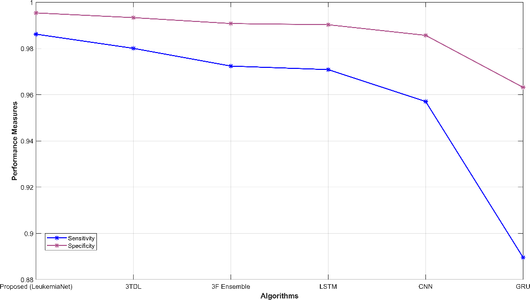
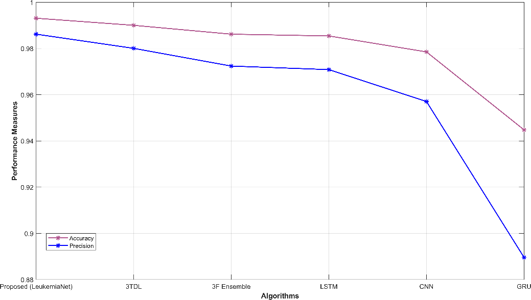
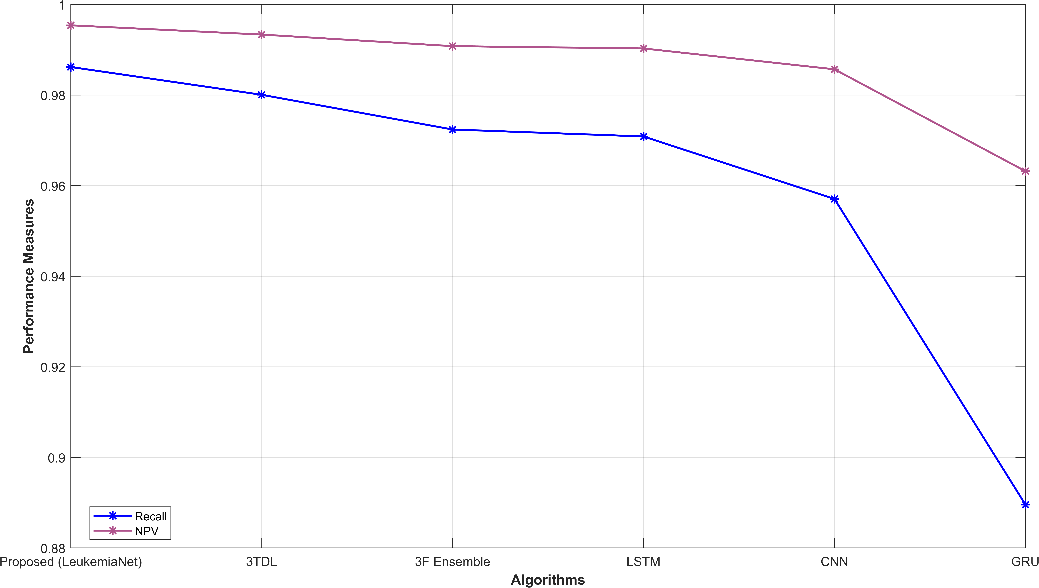
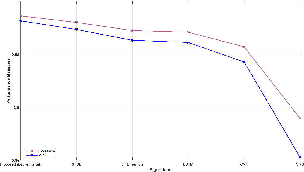
Table I presents a comprehensive performance analysis of various methods employed for leukemia detection, including the proposed model known as LeukemiaNet, as well as other existing approaches. The results for the proposed LeukemiaNet model are notably impressive, with a sensitivity of 0.986, specificity of 0.995, and an accuracy of 0.993. Additionally, the model demonstrates a high precision of 0.986 and recall of 0.986, resulting in an F-measure of 0.986. The NPV is measured at 0.995, highlighting its capacity to accurately predict negative cases, while the FPR is remarkably low at 0.005, indicating minimal false-positive results. Furthermore, the FNR is 0.014, signifying a low rate of false negatives, and the MCC attains a substantial value of 0.982, affirming the model’s effectiveness in leukemia detection. Comparatively, the LeukemiaNet model consistently outperforms alternative approaches including existing models across all evaluation criteria. These results collectively emphasize the superior performance and precision of the proposed model, highlighting its potential to accurately identify leukemia cases, a crucial advancement in the field of medical diagnosis. The successful diagnosis of leukaemia by the system is largely due to the integration of HPSBI inside the framework, which is essential to obtaining the exceptional accuracy seen in the suggested model.
Table I: Overall Performance Analysis
| Method | Sen | Spec | Acc | Pre | Rec | F-M | NPV | FPR | FNR | MCC |
| Proposed (LeukemiaNet) | 0.986 | 0.995 | 0.993 | 0.986 | 0.986 | 0.986 | 0.995 | 0.005 | 0.014 | 0.982 |
| 3TDL (Paper 2) | 0.98 | 0.993 | 0.99 | 0.98 | 0.98 | 0.98 | 0.993 | 0.007 | 0.02 | 0.973 |
| 3F ensemble (Paper 1) | 0.972 | 0.991 | 0.986 | 0.972 | 0.972 | 0.972 | 0.991 | 0.009 | 0.028 | 0.963 |
| LSTM | 0.971 | 0.99 | 0.985 | 0.971 | 0.971 | 0.971 | 0.99 | 0.01 | 0.029 | 0.961 |
| CNN | 0.957 | 0.986 | 0.979 | 0.957 | 0.957 | 0.957 | 0.986 | 0.014 | 0.043 | 0.943 |
| GRU | 0.89 | 0.963 | 0.945 | 0.89 | 0.89 | 0.89 | 0.963 | 0.037 | 0.11 | 0.853 |
4.3. Graphical Representation
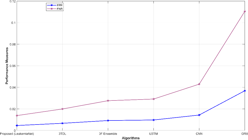
Fig. 3 provides a comprehensive visual representation of various performance metrics. Subfigures (a) and (b) display sensitivity, specificity, accuracy, and precision, offering insights into the model’s ability to correctly classify leukemia cases. Subfigure (c) showcases recall and NPV, highlighting the model’s capability to identify true positives and negatives. In subfigure (d), f-measure and MCC illustrate the balance between precision and recall. Finally, subfigure (e) depicts FPR and FNR, emphasizing the model’s efficiency in minimizing false classifications. These visualizations offer a holistic view of the model’s performance across a range of critical evaluation criteria.
(a)
(b)
(c)
(d)
(e)
Figure 3: Graphical representation (a) sensitivity, specificity, (b) accuracy, precision, (c) recall, NPV, (d) f-measure, MCC, (e) FPR, FNR
 |  |  |  |
| (a) | (b) | (c) | (d) |
 |  |  |  |
| (a) | (b) | (c) | (d) |
 |  |  |  |
| (a) | (b) | (c) | (d) |
 |  |  |  |
| (a) | (b) | (c) | (d) |
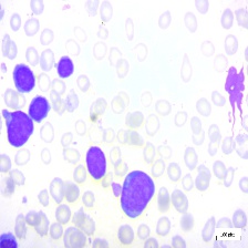
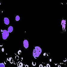
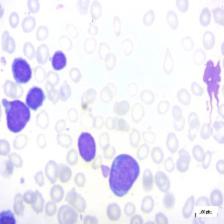
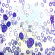
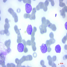
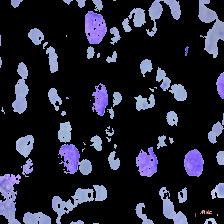
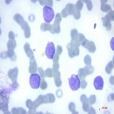
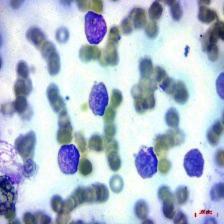
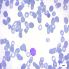
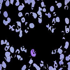
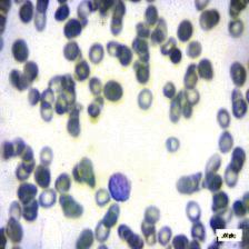
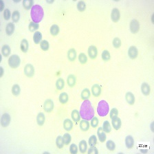
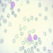
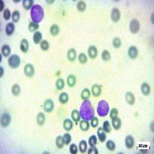
Figure 4: Sample images
Fig. 4 displays sample images, with (a) illustrating different malignancy stages, (b) demonstrating custom CIS application, (c) showcasing Gaussian blur, and (d) depicting histogram equalization.
5. Conclusion
Malignant blood cancer leukaemia posed a serious threat to one’s health, especially if it wasn’t detected early and correctly. This study used cutting-edge methods and technology to build a thorough strategy for detecting leukaemia cancer. For image augmentation, GAN was used to increase the model’s resilience and generalizability. A series of preprocessing techniques followed the pattern. While Histogram Equalisation increased image contrast, enhancing image contrast, and reducing noise, Gaussian Blur was used to enhance image quality and facilitate further studies. A customized CIS technique for accurate cell identification was a crucial component of this architecture. Following segmentation, a variety of characteristics including shape-, texture-, and intensity-based descriptors were collected from these cells. The LeukemiaNet model, a combination of CNN and an O-LSTM network, served as the framework’s central component. The hybrid algorithm HPSBI was used to optimise the weights of the LSTM network, ensuring the model’s accuracy and efficacy in leukaemia diagnosis. MATLAB was used to implement the suggested model. The model achieved an impressive accuracy rate of 99.3%.
Reference
- Bukhari, M., Yasmin, S., Sammad, S., El-Latif, A. and Ahmed, A., 2022. A deep learning framework for leukemia cancer detection in microscopic blood samples using squeeze and excitation learning. Mathematical Problems in Engineering, 2022.
- Shaheen, M., Khan, R., Biswal, R.R., Ullah, M., Khan, A., Uddin, M.I., Zareei, M. and Waheed, A., 2021. Acute myeloid leukemia (AML) detection using AlexNet model. Complexity, 2021, pp.1-8.
- Ahmed, N., Yigit, A., Isik, Z. and Alpkocak, A., 2019. Identification of leukemia subtypes from microscopic images using convolutional neural network. Diagnostics, 9(3), p.104.
- Kumar, D., Jain, N., Khurana, A., Mittal, S., Satapathy, S.C., Senkerik, R. and Hemanth, J.D., 2020. Automatic detection of white blood cancer from bone marrow microscopic images using convolutional neural networks. IEEE Access, 8, pp.142521-142531.
- Khandekar, R., Shastry, P., Jaishankar, S., Faust, O. and Sampathila, N., 2021. Automated blast cell detection for Acute Lymphoblastic Leukemia diagnosis. Biomedical Signal Processing and Control, 68, p.102690.
- Al-jaboriy, S.S., Sjarif, N.N.A., Chuprat, S. and Abduallah, W.M., 2019. Acute lymphoblastic leukemia segmentation using local pixel information. Pattern Recognition Letters, 125, pp.85-90.
- Loey, M., Naman, M. and Zayed, H., 2020. Deep transfer learning in diagnosing leukemia in blood cells. Computers, 9(2), p.29.
- Mishra, S., Majhi, B. and Sa, P.K., 2019. Texture feature-based classification on microscopic blood smear for acute lymphoblastic leukemia detection. Biomedical Signal Processing and Control, 47, pp.303-311.
- Mohammed, Z.F. and Abdulla, A.A., 2021. An efficient CAD system for ALL cell identification from microscopic blood images. Multimedia Tools and Applications, 80(4), pp.6355-6368.
- Bibi, N., Sikandar, M., Ud Din, I., Almogren, A. and Ali, S., 2020. IoMT-based automated detection and classification of leukemia using deep learning. Journal of healthcare engineering, 2020, pp.1-12.
- Di Ruberto, C., Loddo, A. and Putzu, L., 2020. Detection of red and white blood cells from microscopic blood images using a region proposal approach. Computers in biology and medicine, 116, p.103530.
- Liu, Y. and Long, F., 2019. Acute lymphoblastic leukemia cells image analysis with deep bagging ensemble learning. In ISBI 2019 C-NMC Challenge: Classification in Cancer Cell Imaging: Select Proceedings (pp. 113-121). Singapore: Springer Singapore.
- Prellberg, J. and Kramer, O., 2019. Acute lymphoblastic leukemia classification from microscopic images using convolutional neural networks. In ISBI 2019 C-NMC Challenge: Classification in Cancer Cell Imaging: Select Proceedings (pp. 53-61). Springer Singapore.
- Jha, K.K. and Dutta, H.S., 2019. Mutual information-based hybrid model and deep learning for acute lymphocytic leukemia detection in single cell blood smear images. Computer methods and programs in biomedicine, 179, p.104987.
- Boldú, L., Merino, A., Acevedo, A., Molina, A. and Rodellar, J., 2021. A deep learning model (ALNet) for the diagnosis of acute leukaemia lineage using peripheral blood cell images. Computer Methods and Programs in Biomedicine, 202, p.105999.
- Hossain, M.A., Islam, A.M., Islam, S., Shatabda, S. and Ahmed, A., 2022. Symptom based explainable artificial intelligence model for leukemia detection. IEEE Access, 10, pp.57283-57298.
- Sampathkumar, A., Rastogi, R., Arukonda, S., Shankar, A., Kautish, S. and Sivaram, M., 2020. An efficient hybrid methodology for detection of cancer-causing gene using CSC for micro array data. Journal of Ambient Intelligence and Humanized Computing, 11, pp.4743-4751.
- Das, P.K. and Meher, S., 2021. An efficient deep convolutional neural network-based detection and classification of acute lymphoblastic leukemia. Expert Systems with Applications, 183, p.115311.
- Jiang, Z., Dong, Z., Wang, L. and Jiang, W., 2021. Method for diagnosis of acute lymphoblastic leukemia based on ViT-CNN ensemble model. Computational Intelligence and Neuroscience, 2021.
- Baig, R., Rehman, A., Almuhaimeed, A., Alzahrani, A. and Rauf, H.T., 2022. Detecting malignant leukemia cells using microscopic blood smear images: a deep learning approach. Applied Sciences, 12(13), p.6317.
- Ansari, S., Navin, A.H., Sangar, A.B., Gharamaleki, J.V. and Danishvar, S., 2023. A customized efficient deep learning model for the diagnosis of acute leukemia cells based on lymphocyte and monocyte images. Electronics, 12(2), p.322.
- Dasariraju, S., Huo, M. and McCalla, S., 2020. Detection and classification of immature leukocytes for diagnosis of acute myeloid leukemia using random forest algorithm. Bioengineering, 7(4), p.120.
- Acharya, V. and Kumar, P., 2019. Detection of acute lymphoblastic leukemia using image segmentation and data mining algorithms. Medical & biological engineering & computing, 57, pp.1783-1811.
- Inbarani H, H. and Azar, A.T., 2020. Leukemia image segmentation using a hybrid histogram-based soft covering rough k-means clustering algorithm. Electronics, 9(1), p.188.
- Abunadi, I. and Senan, E.M., 2022. Multi-method diagnosis of blood microscopic sample for early detection of acute lymphoblastic leukemia based on deep learning and hybrid techniques. Sensors, 22(4), p.1629.
- Dataset taken from: “https://www.kaggle.com/datasets/mehradaria/leukemia”, dated 05/10/2023.
Cite This Work
To export a reference to this article please select a referencing stye below:

Academic Master Education Team is a group of academic editors and subject specialists responsible for producing structured, research-backed essays across multiple disciplines. Each article is developed following Academic Master’s Editorial Policy and supported by credible academic references. The team ensures clarity, citation accuracy, and adherence to ethical academic writing standards
Content reviewed under Academic Master Editorial Policy.