Abstract
In renewable energy, precise wind power forecasting (WPF) is critical for grid stability. This paper introduces a novel deep learning (DL) ensemble method for enhanced accuracy. The proposed methodology encompasses a comprehensive pre-processing phase, involving data cleaning and normalization through Box-Cox transformation, as well as data imputation to handle missing values. Feature extraction leverages statistical attributes such as skewness, kurtosis, autocorrelation, and fundamental statistics like mean, median, standard deviation, mode, variance, kurtosis, skewness, moment, and interquartile range. The use of Principal Component Analysis (PCA) minimises dimension while retaining crucial data. To further enhance model performance, a hybrid feature selection algorithm, named Hybrid Male Mayflies and Motherly Chicks (HMMMC), is employed. HMMMC synergizes the chicken swarm optimization algorithm (CSO) and mayfly optimization algorithm (MA) to identify the most relevant features for WPF. The core of our method is the Hybrid Sequential Forest (HybSeqFor), which integrates Random Forest (RF), Long Short-Term Memory (LSTM) networks, and Convolutional Neural Networks (CNN). This ensemble produces higher forecasting accuracy by efficiently capturing both spatial and temporal interdependence in wind power data. The proposed model is implemented using MATLAB.
Keywords- WPF; DL; PCA; HMMMC; HybSeqFor; CNN; LSTM; RF.
1. Introduction
WPF plays a pivotal role in the modern energy landscape, especially as the world moves towards a more sustainable and renewable future. The harnessing of wind energy has seen remarkable growth in recent years, making it a leading source of clean, renewable power [1,2]. To address these challenges, accurate WPF has become an essential tool for ensuring the reliability and stability of power systems [3,4]. One of the fundamental characteristics of wind power generation is its dependency on meteorological conditions, primarily wind speed and direction. Unlike traditional power generation from fossil fuels or nuclear sources, wind power production is subject to the whims of nature. Efficient electricity generation from wind turbines depends on a steady and ample wind source [5,6]. As the wind varies in strength and direction over time, accurately forecasting the wind’s behavior becomes crucial for efficient power generation and grid management.
WPF addresses the critical issue of predicting how much power will be generated by wind turbines at a specific point in the future [7]. This prediction is essential for various aspects of power system operation, including grid planning, scheduling, and real-time balancing [8,9]. The ability to anticipate wind power generation helps grid operators make informed decisions about how to meet electricity demand, allocate resources, and maintain the stability of the grid. In today’s power systems, three main forecasting challenges related to wind power exist: load forecasting, price forecasting, and renewable energy source forecasting [10]. Among these, WPF stands out due to the unique characteristics of wind as a renewable energy source. Unlike solar power, which exhibits more predictable daily patterns, wind power is highly variable, intermittent, and stochastic in nature.
WPF is performed over different time horizons, depending on the specific application [11]. Short-term WPF is crucial for grid operators to make real-time decisions about power generation and load balancing. The medium-term horizon extends from a few hours to several days ahead. Long-term forecasts extend beyond several days, often covering weeks, months, or even years. Accurate short-term and medium-term wind power forecasting (WPF) is essential for maintaining grid stability and optimizing resource utilization [12,13]. WPF relies on deep learning techniques like recurrent neural networks (RNN) and CNN. These models analyze historical weather and turbine data to capture complex temporal and spatial wind behavior, improving prediction accuracy [14,15]. Precise forecasts support efficient energy market operations and grid management, reducing costs and facilitating the integration of wind energy for a greener and sustainable future.
The primary focus of this research is to:
- In data preprocessing, a notable aspect involves applying the Box-Cox transformation for data normalization and ensuring robustness in handling missing values through data imputation techniques.
- To enhance model performance, presents a novel hybrid feature selection algorithm, HMMMC, which synergizes CSO and MA to identify the most pertinent features for WPF.
- To the core of our approach, HybSeqFor, combines CNN, LSTM, and RF capturing both spatial and temporal dependencies in wind power data, thereby significantly improving forecasting accuracy.
The rest of this paper is arranged as: Section 2 discusses about the literature works reviews regarding WPF. Section 3 talks about the WPF using ensemble classifiers: architectural description. Section 4 manifests about the recorded results. This paper is concluded in section 5.
2. Literature Review
In 2020, Ahmadi et al. [16] pioneered the creation of three six-month-ahead WPF models using tree-based learning algorithms. Model 1 relied on the mean and standard deviation of 10-minute wind speed data at 40 meters. Model 2, on the other hand, delved into the influence of different sampling intervals (1-hour, 12-hour, and 24-hour) at the same height. Model 3 ventured into height extrapolation, incorporating data from heights of 30 meters and 10 meters to predict wind speeds at 40 meters. In 2021, Yang et al. [17] introduced an enhanced Fuzzy C-means Clustering Algorithm for day-ahead wind power prediction. Their innovation focused on more accurate cluster center selection through minimum distance principles. This improvement led to better clustering of turbines with similar power output patterns, aiding in creating representative power curves for assessing wind turbine performance. Additionally, Dong et al. [18] in the same year introduced a novel hybrid forecasting approach involving decomposition, Bernstein polynomials, and a mixture of Gaussians, optimizing model parameters with a population-based multi-objective state transition algorithm, contributing to wind power prediction advancements.
Furthermore, in 2022, Rayi et al. [19] introduced an innovative hybrid time series forecasting model for precise wind power prediction. This model cleverly fused VMD with Deep Learning Mixed Kernel ELM Autoencoder (MKELM-AE). What set this approach apart from other deep learning neural network models was its ability to avoid nonconvex optimization issues, reduce training time, and deliver precise output weight solutions through generalized least squares. Additionally, in 2020, Ko et al. [20] introduced a pioneering deep residual network designed to enhance time-series forecasting models, particularly vital for reliable power grid operation in the context of high renewable energy contributions. Their approach tackled potential overfitting issues associated with stacked bidirectional long short-term memory (Bi-LSTM) layers. It seamlessly integrated multi-level residual networks (MRN), DenseNet, long and short Bi-LSTM networks, and advanced activation functions, resulting in superior prediction accuracy and parameter efficiency. In 2022, Ahmad et al. [21] introduced the STSR-LSTM model, a deep sequence-to-sequence long short-term memory regression, tailored for time-series wind power forecasting. This innovative approach significantly enhanced feature reliability and overall predictive performance. Meanwhile, in 2020, Sun et al. [22] pioneered the Multi-Distribution Ensemble (MDE) probabilistic framework for wind power forecasting. This strategy harnessed various predictive distributions and employed competitive and cooperative methods to create probabilistic forecasts for different timeframes, integrating Gaussian, gamma, and Laplace distribution-based models while optimizing ensemble parameters during training.
In 2019, Du et al. [23] unveiled a highly effective hybrid wind energy prediction model encompassing three critical stages: the decomposition of wind energy series, the implementation of an improved wavelet neural network, and rigorous testing. Empirical results showcased significantly lower mean absolute percent errors compared to alternative models, underscoring the model’s efficacy in wind energy prediction. Additionally, in 2020, Wang et al. [24] introduced a hybrid WPF approach known as BMA-EL, artfully blending Bayesian model averaging and ensemble learning techniques. This innovative methodology commenced with Self-Organizing Map (SOM) clustering and K-fold cross-validation, creating diverse training subsets from meteorological data. These subsets served as the foundation for training three distinct base learners: Backpropagation Neural Network (BPNN), Radial Basis Function Neural Network (RBFNN), and Support Vector Machine (SVM). Furthermore, in 2020, Liu et al. [25] proposed the Chinese Wind Power Generation model, a hybrid approach that seamlessly integrated Wavelet Decomposition (WD) for data stabilization and Long Short-Term Memory neural network (LSTM) for predicting national wind power output.
2.1. Problem Statement
Challenges within the field of WPF encompass the inherently volatile and sporadic nature of wind patterns, the intricacy of handling diverse meteorological variables in data, the demand for precise predictions across short and long-term timeframes, inherent uncertainties within predictive models, and geographical variations in wind patterns [1]. These challenges may lead to inaccurate and unreliable wind power forecasting results, hindering wind energy grid integration [16]. The challenges in WPF, including variability, data complexity, short-term and long-term forecasting requirements, model uncertainty, and spatial variability, can be effectively addressed through an Ensemble Deep Learning approach. By combining Convolutional Neural Networks (CNNs), Long Short-Term Memory (LSTM) networks, and Random Forest, a comprehensive solution can be developed. An Ensemble Deep Learning approach offers a comprehensive solution to the multifaceted challenges of WPF, leading to improved accuracy, reliability, and adaptability in forecasting wind power generation for grid operations and renewable energy integration.
3. Proposed Methodology
WPF is an essential method for estimating the potential electricity output from wind energy sources in the future. As wind energy production is unpredictable and weather-dependent, accurate forecasting is crucial for grid operation. This helps with grid management, energy trading, and guaranteeing a steady supply of electricity from renewable sources. This work developed an ensembled DL for WPF employs models to enhance wind power predictions. This approach leverages the strengths of each model and uses a meta-heuristic optimization method to improve forecast accuracy. Fig. 1 depicts the overall proposed architecture.
Figure 1: Overall Proposed Architecture
3.1. Dataset Description
This project aims to forecast wind turbine power generation using key variables like wind speed, wind direction, month, and hour. With a Wind Turbine Power Prediction-GBTRegressor PySpark dataset [26] comprising 50,530 observations, this project not only addresses power prediction but also showcases expertise in handling big data. To effectively manage and analyze this large-scale dataset, the PySpark library is employed, highlighting the ability to work with extensive data sets. The dataset includes critical labels such as Date/Time for temporal, LV ActivePower (kW) indicating actual power output, Wind Speed (m/s), Wind Direction (°), and Theoretical_Power_Curve (KWh) serving as a reference for optimal power production. This project exemplifies data science skills in handling, analysing, and predicting wind turbine power generation.
3.2. Pre-processing
In this study, data pre-processing techniques, data cleaning and normalization, have been employed as essential steps to enhance the quality and suitability of the dataset for subsequent analysis and modeling.
3.2.1. Data Cleaning
In WPF, data cleansing is a crucial step that improves the precision and dependability of predictions. To estimate future energy output, WPF significantly relies on previous data, particularly wind speed, direction, and other meteorological factors. But a lot of the time, this data comes with a lot of problems. First and foremost, data validation is crucial. It entails locating and fixing data points that deviate from expected ranges or have unlikely values. The next critical step is to deal with missing data. Gaps can be filled using methods like interpolation or data from adjacent sources. For locating and managing incorrect data items that can skew forecasts, outlier detection is essential. Data from several sources are synchronised and aligned with one another according to the principle of temporal consistency. Feature engineering entails adding new variables to collect relevant information. At the final, continual quality control processes are required to track data quality over time and adjust to changing circumstances. In WPF, data cleaning is a thorough process that includes feature engineering, data validation, missing value filling, outlier identification, guaranteeing temporal consistency, and continual quality control. In the end, it results in more precise and trustworthy wind power estimates, facilitating effective energy grid integration.
3.2.2. Normalization – Box-Cox Transformation
The process of scaling data to have a common range or distribution is called normalisation. When working with data aspects that have various scales or units, it is especially helpful. The objective is to scale all the variables to the same value, which is normally between 0 and 1, however other scales may also be employed. Data preprocessing statistical techniques like the Box-Cox transformation are utilised in many disciplines like statistics, machine learning, and data analysis. These techniques try to enhance the volume and distribution of data, making it better suited for modelling and analysis. A specific kind of power transformation called the Box-Cox transformation is used to reduce variance and improve the normality of a dataset. It is appropriate for heteroscedastic data, when the distribution of data points differs across various levels of the independent variable. According to Eq. (1), the transformation is described.
(1)
The original data is represented by , and the transformation parameter is altered to determine the best-fit transformation. The Box-Cox transformation is useful when working with data that differs from the presumptions of many statistical models, such as linear regression. In a variety of domains, both normalisation and the Box-Cox transformation are efficient techniques for raising the calibre of data and getting it ready for analysis and modelling.
3.2.3. Data Imputation
A crucial statistical technique used to deal with missing or insufficient data points in a dataset is data imputation. Due to different variables including measurement errors or sensor problems, data can be rife with gaps. The general integrity of the dataset is maintained by using imputation techniques to estimate these missing values based on the information that is currently available. Regression, mean, and median imputation are three often used imputation methods. With mean imputation, the observed data’s mean is used to fill in for a variable’s missing values. While median imputation employs the median, regression imputation predicts missing values by creating a regression model based on other variables in the dataset.
3.3. Feature Extraction
After the data preprocessing phase, the next step in the analysis involves feature extraction. Various statistical and higher-order statistical features are computed from the data to capture important characteristics and features. Here are some of the key features extracted:
3.3.1. Mean
The mean is calculated by dividing the sum by the count. This is mathematically shown in Eq. (2).
(2)
3.3.2. Median
In datasets with an odd number of values, the median is the middle value. For even sets, it’s the average of two middles, per Eq. (3).
(3)
Thus, a set of data can be divided into two sections using the median. It is necessary to arrange the set’s components in ascending order in order to determine the set’s median. Then locate the midpoint.
3.3.3. Standard Deviation
Standard deviation (SD) measures data deviation from the mean. Low SD means values are close; high SD, they’re spread. This is mathematically shown in Eq. (4).
SD ( (4)
Where is the input value (pre-processed data, is the mean and N represents number of total elements.
3.3.4. Mode
The most frequent value within a dataset is identified by the mode, a statistical measure of central tendency. Unlike the mean and median, which emphasise average or midway values, respectively, it is different. Whether the dataset contains numerical values or categorical data, it is arranged in either ascending or descending order to establish the mode. The mode is then determined as the value that appears the most frequently. The mode offers important insights into the features of the dataset and is especially helpful when identifying the most common value or category within a dataset.
3.3.5. Variance
Variance measures numerical variation, indicating how data points deviate from the mean and each other, as in Eq. (5).
(5)
3.3.6. Moment
The Euclidean separation between the centroid and boundary points is the order sequence . is the index of the Fourier descriptors and represents the total number of boundary coefficients. Eq. (6) – Eq. (8) can be used to calculate the second order central moment and second order contour sequence moment .
(6)
(7)
(8)
3.3.7. Interquartile Range (IQR)
IQR is a statistical measure used to understand the spread or dispersion of data in a dataset. It is calculated by finding the difference between the third quartile () and the first quartile (). Quartiles split data into four equal parts and are robust to outliers. It is often used in box-and-whisker plots to visualize the variability and distribution of data, helping analysts identify trends and anomalies. The formula for inter-quartile range is given as per Eq. (9).
(9)
3.3.8. Kurtosis
A statistical measure known as kurtosis defines the pattern of a set of values’ distribution. The peakedness or flatness of the data in relation to a normal distribution is measured. Zero kurtosis denotes a normal distribution, while positive kurtosis denotes a more pronounced peak and negative kurtosis denotes a flatter distribution. In financial and economic analysis, kurtosis is frequently used to describe the distribution of returns from investments or financial assets. High kurtosis may suggest a higher level of tail risk, or the risk of extreme events, such as big losses, in these applications, where it is used to measure the investment’s risk. This is demonstrated quantitatively in Eq. (10).
(10)
3.3.9. Skewness
A statistical measure known as skewness identifies an asymmetrical distribution of values. It gauges how far the numbers deviate from the mean by tilting them to one side or the other. The values in a normal distribution are symmetrical around the mean because the skewness is zero. Having a positive skewness implies that the values are moved to the right or that the right side of the distribution has a long tail, whereas having a negative skewness suggests that the values are shifted to the left or that the left side of the distribution has a long tail. According to Eq. (11), skewness is used to characterise the distribution of data and to spot any asymmetries in the data.
(11)
3.3.10. Auto-correlation
Autocorrelation quantifies signal self-similarity over time, computed as in Eq. (12).
(12)
In Eq. (12), denotes correlation sequences, is the time shift parameter. Autocorrelation gauges vibration signal similarity in this study.
3.3.11. PCA
PCA reduces data dimensionality in WPF while preserving information. Data is normalized, and the covariance matrix is computed as per Eq. (13) and Eq. (14).
(13)
(14)
The optimal number of principal components () is determined by selecting the top eigenvalues. Thresholding is applied to separate significant eigenvalues from noise. This process enhances the representation of underlying data structure Eq. 15 and Eq. 16.
(15)
(16)
The retained eigenvalues () and eigenvectors () are utilized for feature extraction (Eq. 17). Here, is transposed-data, and is transformed-feature. These extracted features are subsequently used for feature selection, enhancing the effectiveness of the overall WPF process.
(17)
3.4. Feature Selection
Following feature extraction, the process of feature selection becomes important for refining the dataset. This study employs advanced hybrid algorithms HMMMC, including CSO and MA.
3.4.1. Hybrid Male Mayflies and Motherly Chicks (HMMMC)
MA is inspired by the unique life cycle of mayflies. Mayflies hatch as mature adults, and their fitness depends on initial traits, not lifespan. CSO mimics chicken swarms’ hierarchical structure and food-searching behavior. Chickens are categorized as roosters, hens, or chicks based on fitness. Hierarchies and mother-child relationships are updated iteratively. Chickens cooperate and compete for food. CSO has an initialization step and assumptions about hen numbers, mother hen selection, and chick numbers.
3.4.1.1. Male Mayflies Movement
Male mayflies gather in swarms, adjusting their positions based on personal experience and their neighbours’ movements. This behavior is mathematically represented as chicks following their mother in CSO. Eq. (18) is used to update the male mayflies’ positions.
(18)
Here, represents mayfly male current position and calculate velocity position, the next position attained. Male mayflies hover above the water surface to enhance their speed. However, the algorithm finds only local optimal solutions, and Eq. (19) calculates their velocity to improve their movement performance.
(19)
Where represents the velocity mayfly in dimension j, The positive attraction constants, denoted as quantify the contributions of cognitive and social components.A constant coefficient limits how visible a mayfly is to other people. Additionally, corresponds to the optimal position inspected by mayfly i, andrepresents the position of the best male mayfly in Eq. (20) illustrates the minimization problem for .
= (20)
Here, fitness reflects solution quality, while represents Manhattan distance between and , and for and . The Manhattan-based distance with CSO based Hybridization has been taken into account in this algorithm. In comparison to the conventional MA and CSO optimization, this hybrid metaheuristic approach improves optimization performance. One of the key advantages of using Manhattan distance is its simplicity. Manhattan distance only requires simple arithmetic calculations. This makes it easier to implement and computationally faster. A single extreme value in the data will not greatly affect the calculated distance. The use of the Manhattan distance in the algorithm provides a way to balance the trade-off between energy efficiency and reliability, allowing the algorithm to make efficient and effective decisions in a D2D communication network. The Manhattan distance as shown in Eq. (21) in n-dimensional space from two locations and is the total of the distances in each dimension.
(21)
Here, represents the velocity of the current-position. Nuptial-dance performance by best-mayfly introduces randomness into the algorithm, mathematically represented as Eq. (22). The nuptial dance coefficient gradually decreases as where is the initial value, is the current iteration count, and is a random number in [0, 1]. To enhance solution convergence in the male mayfly update phase, the gravitational coefficient has been considered.
(22)
3.4.1.2. Female Mayflies Movement
Mayflies that are female do not cluster together. Instead, they fly in the direction of males to mate. The algorithm runs the risk of getting stuck in a sub-optimal solution and may not produce the most optimal solution possible. In order to overcome this problem, female mayflies’ movement is based on the narrowed exploration of
CSO. Eq. (23) shows the updating of female mayflies with addition of velocity.
(23)
Female mayfly position at time T, denoted as , is improved by calculating its velocity. This process involves the mutual attraction between optimal male and female performers.
= (24)
In Eq. (24), represents the position, velocity female-mayfly dimension at . Constants and are predefined and correspond to the coefficients for obviousness, and denotes male and female mayflies Manhattan distance, random walk coefficient comes into play when a female mayfly doesn’t find a male attractive, causing it to fly randomly. The variable o represents a random value within the range [-1, 1].
3.4.1.3. Crossover
Crossover begins by selecting the best male and female mayflies based on their fitness values for pairing. Eq. (25), and Eq. (26), respectively, prove this in a mathematical manner.
(25)
(26)
Male and female represent the parent mayflies, falls between 0 and 1. Initial speeds of the offspring are 0.
3.5. Wind-Power Forecasting via Hybrid Sequential Forest (HybSeqFor)
After selecting the optimal features, WPF employs a hybrid approach that leverages advanced learning techniques. Fig. 2 illustrates HybSeqFor, a model for wind power forecasting. It combines CNN for spatial analysis, LSTM for temporal dependencies, and RF for ensemble predictions, enhancing accuracy. By combining the strengths of these models, the forecasting system enhances the accuracy and reliability of wind power predictions.
Figure 2: HybSeqFor: Enhanced Wind Power Forecasting with Combined Models
3.5.1. CNN
CNN, a deep ANN, excels in extracting spatial data for forecasting.
3.5.1.1. Convolutional layer
In the convolutional layer, the convolution operation replaces matrix multiplication, sharing parameters for efficiency, and is defined as per Eq. (27).
(27)
Where represents the kernel weight at position (i, l), represents pixel value at and defines kernel’s size.
3.5.1.2. ActivationFunction
ReLU in CNN prevents gradient vanishing and hastens training; Eq. (28) clarifies.
(28)
3.5.1.3. Pooling Layer
The pooling layer, often max pooling, reduces network complexity and concentrates data. Eq. (29) illustrates max pooling.
(29)
Where rounds up a number, and are output feature map dimensions, and are input dimensions, feature map padding, max pooling kernel size, max pooling kernel stride.
3.5.1.4. Fully Connected Layer
Fully connected layers, also known as dense layers, ensure every neuron connects with those in the layers above and below. Each link between neurons has a learnable weight that is modified during training to improve the performance of the network. To find non-linear patterns and correlations in the input data, fully connected layers are used. These layers can record intricate feature interactions. The following formula can be used to calculate the outputs of a layer with M input neurons and N output neurons that is fully connected:
The output value is calculated for each output neuron by adding the weighted inputs from all input neurons and using an activation function,
(30)
In Eq. (30), is output of neuron, is activation function applied element-wise to weighted sum of inputs, is weighted sum of inputs to neuron, is weight associated with connection between input neuron and output neuron, is input value of neuron, is bias term for neuron.
3.5.2. LSTM
LSTM, designed to tackle gradient issues, excels in time-series data analysis, capturing long-term dependencies. Its cell manages memory transfer with input, update, forget, and output gates, each serving a distinct purpose. The input gate, defined in Eq. 31, determines data to enter the cell.
= (31)
The vectors are multiplied element by element by operator . Eq. (32) represents the forget gate.
(32)
The update gate changes the state of the cell and is theoretically represented by Eq. (33) and Eq. (34),
= (33)
= (34)
Output gate updates prior step’s hidden layer using Eq. (35) and (36).
= (35)
(36)
3.5.3. RF
Random Forest (RF) is an ensemble method combining decision trees. It works as follows: (i) repeatedly resample the initial training data, (ii) randomly select features for each resample, (iii) create a decision tree for each resample, and (iv) combine these trees into one. RF leverages tree variance for classification, with each tree casting a vote on class membership. RF excels due to its ability to handle large datasets, numerous input variables, generate unbiased error estimates, assess variable significance, compute case distances, and perform consistently across noisy datasets. In classification, it builds trees from samples, splitting nodes optimally to maximize purity. Impurity is measured using the Gini-Index, as in Eq. (37).
(37)
The Gini index determines the probability that a randomly selected element would be incorrectly labelled if it were done so in accordance with the distribution of classes in the set. When building each decision tree, the quality of splits is frequently assessed using the Gini index as a criterion. The optimal split in a decision tree minimizes the Gini index. The technique seeks to divide each node’s data points into homogeneous groups using the Gini index as the splitting criterion, increasing the random forest’s overall predicting accuracy.
4. Result and Discussion
4.1. Experimental Setup
The MATLAB-based proposed model is evaluated against established models including K-nearest neighbour (KNN), Artificial Neural Network (ANN), Random Forest (RF), Long Short-Term Memory (LSTM), and Convolutional Neural Network (CNN). Performance assessment employs metrics such as NMSE, MAE, RMSE, Correlation, and R-square.
4.2. Performance Metrics
- NMSE – It assesses the goodness of fit of a model by comparing the squared differences between actual and predicted values with the squared differences between actual values and their mean. It provides a normalized measure of the mean squared error, where a lower NMSE indicates a better model fit. It is calculated as per Eq. (38).
(38)
- MAE – It calculates the average absolute differences between actual and predicted values. It provides a straightforward measure of prediction accuracy, with lower MAE values indicating better model performance. It is calculated as per Eq. (39).
(39)
- RMSE – It is a measure of prediction accuracy, emphasizing larger errors. It is calculated as per Eq. (40).
(40)
- Correlation – Correlation quantifies the linear association between variables, ranging from -1 (perfect negative) to +1 (perfect positive), with 0 indicating no correlation. It is calculated as per Eq. (41).
(41)
- R-square – R-squared quantifies how much of the dependent variable’s variance is accounted for by the model, indicating goodness-of-fit. It is calculated as per Eq. (42).
(42)
4.3. Proposed model overall performance
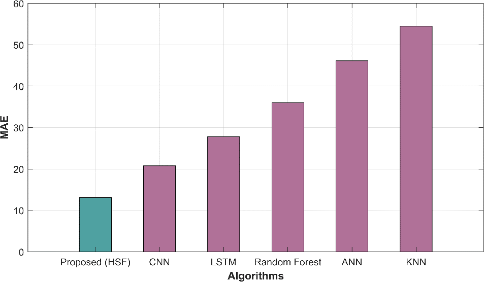
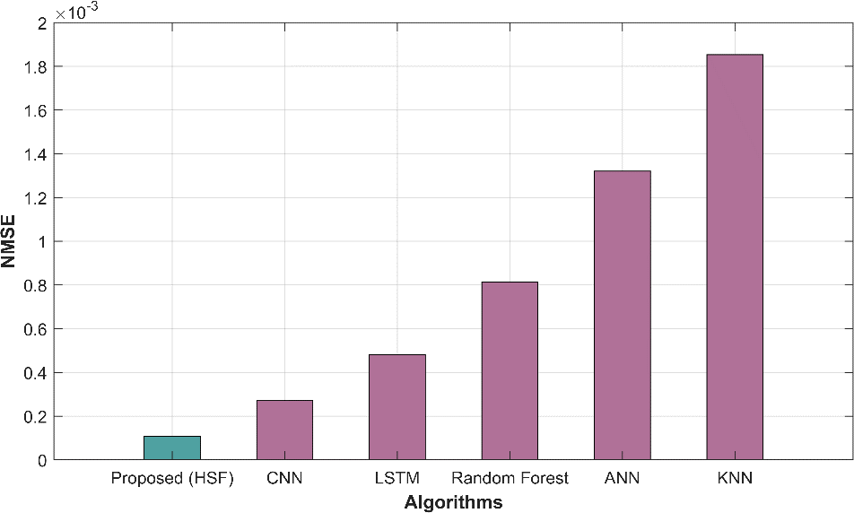
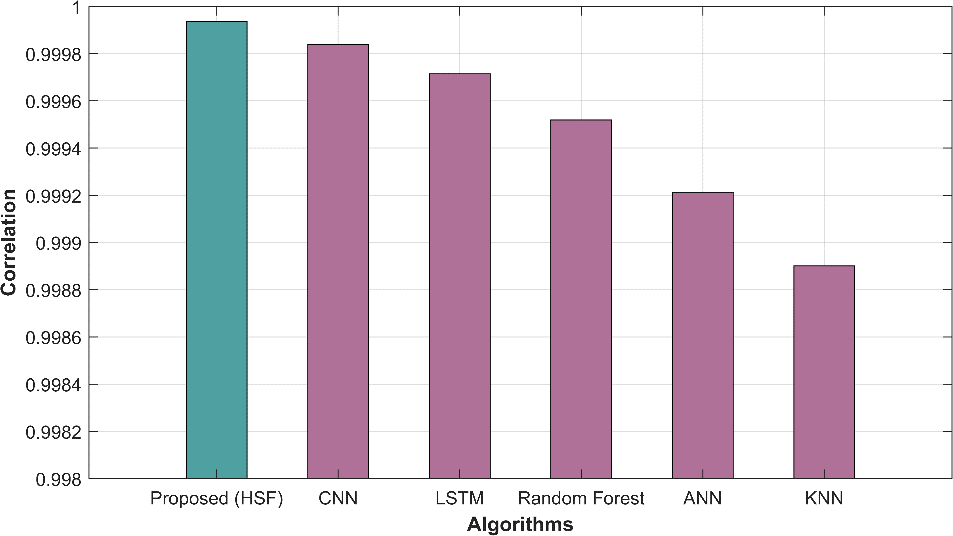
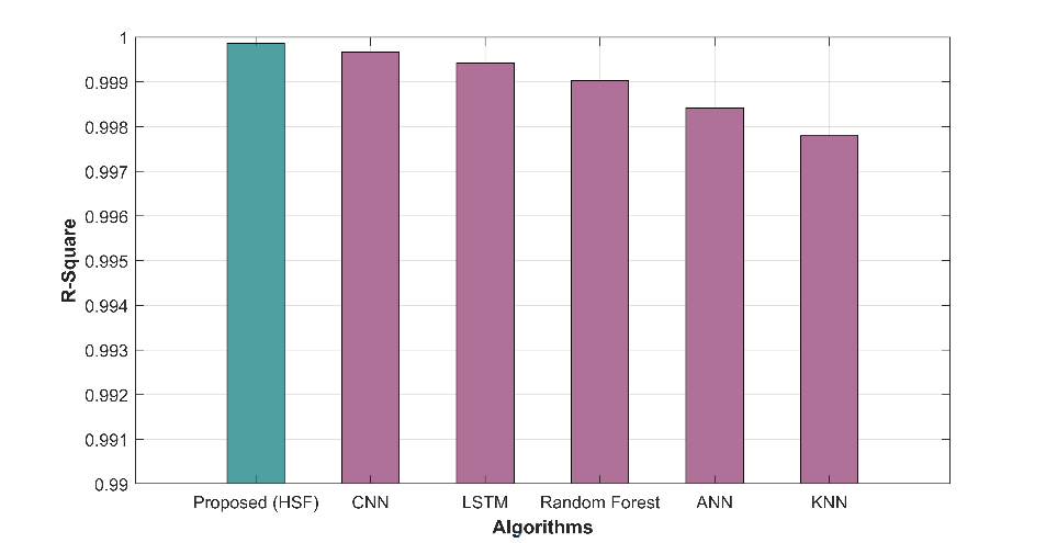
In table 1, several methods have been evaluated based on various performance metrics for a specific task. The metrics used help us assess the accuracy and quality of predictions made by each method. The proposed HSF method demonstrates outstanding performance with a remarkably low MAE of 13.122 and RMSE of 15.217, indicating its superior accuracy in predicting the target variable compared to other methods. The NMSE of 0.0001 indicates minimal prediction errors, while the high correlation (0.99993) and R-squared (0.9998) values highlight strong linear relationships. In contrast, traditional methods such as CNN, LSTM, RF, ANN, and KNN exhibit progressively higher MAE and RMSE values, indicating comparatively lower predictive accuracy. The NMSE values for these methods are also higher, implying larger prediction errors. Additionally, the correlation and R-square values for these methods are lower than proposed HSF, signifying weaker linear relationships between predictions and actual values.
Table 1: Overall performance metrics
| Methods | MAE | RMSE | NMSE | Correlation | R-square |
| Proposed HSF | 13.122 | 15.217 | 0.0001 | 0.99993 | 0.9998 |
| CNN | 20.776 | 24.141 | 0.0002 | 0.99984 | 0.9996 |
| LSTM | 27.776 | 32.212 | 0.0004 | 0.99971 | 0.9994 |
| Random Forest | 35.996 | 41.768 | 0.0008 | 0.99951 | 0.9990 |
| ANN | 46.141 | 53.335 | 0.0013 | 0.99921 | 0.9984 |
| KNN | 54.471 | 63.039 | 0.0018 | 0.99890 | 0.9977 |
4.3. Graphical Representation
Figure 2 displays graphical representations of various performance metrics, including MAE, MAPE, MEAN, MSE, RAE, RMSE, and predicted time, offering a comprehensive view of model evaluation.
(a)

(b)
(c)
(d)
(e)
Figure 2: Graphical representation of (a) MAE (b) RMSE (c) NMSE (d) Correlation (e) R-square
In Figure 3, the graph illustrates the alignment between actual wind power generation values and those predicted by the model. It visually assesses the model’s accuracy and its ability to capture real-world wind power patterns and fluctuations.
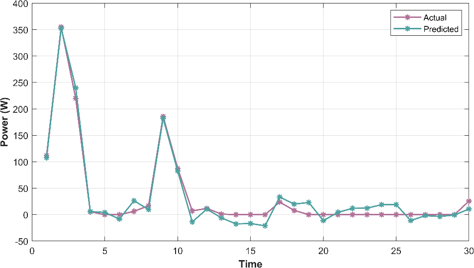
Figure 3: Actual vs Predicted graph
5. Conclusion
In renewable energy, accurate wind power forecasting is crucial for grid stability and resource optimization. This research described a novel method that utilised a group of DL models and a meta-heuristic framework to improve the accuracy of WPF. Data cleaning and normalisation using the Box-Cox transformation, as well as data imputation to accommodate missing values, were all included in the suggested methodology’s thorough pre-processing phase. The statistical properties of skewness, kurtosis, and autocorrelation, as well as the basic statistics of mean, median, standard deviation, mode, variance, kurtosis, skewness, moment, and interquartile range, were used in the feature extraction process. The use of PCA allowed for the reduction of dimensionality while retaining crucial data. HMMMC, a hybrid feature selection approach, was used to further improve model performance. To find the most pertinent features for WPF, HMMMC used CSO with method MA. The core of the method was HybSeqFor, which brought together RF, LSTM, and CNN. The ensemble improved accuracy by capturing spatial and temporal interdependence in wind power data. The suggested model was implemented using MATLAB.
Reference
- Kisvari, A., Lin, Z. and Liu, X., 2021. Wind power forecasting–A data-driven method along with gated recurrent neural network. Renewable Energy, 163, pp.1895-1909.
- Demolli, H., Dokuz, A.S., Ecemis, A. and Gokcek, M., 2019. Wind power forecasting based on daily wind speed data using machine learning algorithms. Energy Conversion and Management, 198, p.111823.
- Duan, J., Wang, P., Ma, W., Fang, S. and Hou, Z., 2022. A novel hybrid model based on nonlinear weighted combination for short-term wind power forecasting. International Journal of Electrical Power & Energy Systems, 134, p.107452.
- Niu, Z., Yu, Z., Tang, W., Wu, Q. and Reformat, M., 2020. Wind power forecasting using attention-based gated recurrent unit network. Energy, 196, p.117081.
- Zhang, Y., Li, Y. and Zhang, G., 2020. Short-term wind power forecasting approach based on Seq2Seq model using NWP data. Energy, 213, p.118371.
- Lin, Z. and Liu, X., 2020. Wind power forecasting of an offshore wind turbine based on high-frequency SCADA data and deep learning neural network. Energy, 201, p.117693.
- Xiong, B., Lou, L., Meng, X., Wang, X., Ma, H. and Wang, Z., 2022. Short-term wind power forecasting based on Attention Mechanism and Deep Learning. Electric Power Systems Research, 206, p.107776.
- Abedinia, O., Lotfi, M., Bagheri, M., Sobhani, B., Shafie-Khah, M. and Catalão, J.P., 2020. Improved EMD-based complex prediction model for wind power forecasting. IEEE Transactions on Sustainable Energy, 11(4), pp.2790-2802.
- Khazaei, S., Ehsan, M., Soleymani, S. and Mohammadnezhad-Shourkaei, H., 2022. A high-accuracy hybrid method for short-term wind power forecasting. Energy, 238, p.122020.
- Li, L.L., Zhao, X., Tseng, M.L. and Tan, R.R., 2020. Short-term wind power forecasting based on support vector machine with improved dragonfly algorithm. Journal of Cleaner Production, 242, p.118447.
- Scarabaggio, P., Grammatico, S., Carli, R. and Dotoli, M., 2021. Distributed demand side management with stochastic wind power forecasting. IEEE Transactions on Control Systems Technology, 30(1), pp.97-112.
- Dong, Y., Zhang, H., Wang, C. and Zhou, X., 2021. Wind power forecasting based on stacking ensemble model, decomposition and intelligent optimization algorithm. Neurocomputing, 462, pp.169-184.
- Wang, C., Zhang, H. and Ma, P., 2020. Wind power forecasting based on singular spectrum analysis and a new hybrid Laguerre neural network. Applied Energy, 259, p.114139.
- Hong, Y.Y. and Rioflorido, C.L.P.P., 2019. A hybrid deep learning-based neural network for 24-h ahead wind power forecasting. Applied Energy, 250, pp.530-539.
- Al-qaness, M.A., Ewees, A.A., Fan, H., Abualigah, L. and Abd Elaziz, M., 2022. Boosted ANFIS model using augmented marine predator algorithm with mutation operators for wind power forecasting. Applied Energy, 314, p.118851.
- Ahmadi, A., Nabipour, M., Mohammadi-Ivatloo, B., Amani, A.M., Rho, S. and Piran, M.J., 2020. Long-term wind power forecasting using tree-based learning algorithms. IEEE Access, 8, pp.151511-151522.
- Yang, M., Shi, C. and Liu, H., 2021. Day-ahead wind power forecasting based on the clustering of equivalent power curves. Energy, 218, p.119515.
- Dong, Y., Zhang, H., Wang, C. and Zhou, X., 2021. A novel hybrid model based on Bernstein polynomial with mixture of Gaussians for wind power forecasting. Applied Energy, 286, p.116545.
- Rayi, V.K., Mishra, S.P., Naik, J. and Dash, P.K., 2022. Adaptive VMD based optimized deep learning mixed kernel ELM autoencoder for single and multistep wind power forecasting. Energy, 244, p.122585.
- Ko, M.S., Lee, K., Kim, J.K., Hong, C.W., Dong, Z.Y. and Hur, K., 2020. Deep concatenated residual network with bidirectional LSTM for one-hour-ahead wind power forecasting. IEEE Transactions on Sustainable Energy, 12(2), pp.1321-1335.
- Ahmad, T. and Zhang, D., 2022. A data-driven deep sequence-to-sequence long-short memory method along with a gated recurrent neural network for wind power forecasting. Energy, 239, p.122109.
- Sun, M., Feng, C. and Zhang, J., 2020. Multi-distribution ensemble probabilistic wind power forecasting. Renewable Energy, 148, pp.135-149.
- Du, P., Wang, J., Yang, W. and Niu, T., 2019. A novel hybrid model for short-term wind power forecasting. Applied Soft Computing, 80, pp.93-106.
- Wang, G., Jia, R., Liu, J. and Zhang, H., 2020. A hybrid wind power forecasting approach based on Bayesian model averaging and ensemble learning. Renewable energy, 145, pp.2426-2434.
- Liu, B., Zhao, S., Yu, X., Zhang, L. and Wang, Q., 2020. A novel deep learning approach for wind power forecasting based on WD-LSTM model. Energies, 13(18), p.4964.
- Dataset taken from: “https://www.kaggle.com/code/akdagmelih/wind-turbine-power-prediction-gbtregressor-pyspark/input”, dated 02/10/2023.
Cite This Work
To export a reference to this article please select a referencing stye below:

Academic Master Education Team is a group of academic editors and subject specialists responsible for producing structured, research-backed essays across multiple disciplines. Each article is developed following Academic Master’s Editorial Policy and supported by credible academic references. The team ensures clarity, citation accuracy, and adherence to ethical academic writing standards
Content reviewed under Academic Master Editorial Policy.