Abstract
The field of analogue electronics has existed for a long time. It forms the fundamental platform for the synthesis of signals in various systems. Resistors, capacitors, and inductors form the elements of a circuit. The characteristics of these components can be studied in a laboratory using the knowledge derived from the first principles. As a researcher in the field, my interest would be to understand the frequency response of the various combinations of the elements, in this case, the resistor-capacitor integral. The main objective of this study is to experimentally measure the frequency response of a simple RC circuit using LabVIEW and observe how changing R and C will affect the result.
Introduction
This lab will involve the study of RC circuits at a basic level. Equations that explain the charging and discharging of capacitors are analyzed. The frequency response of a capacitor is explored using experimental data and a bode plot, and then the theoretical values are compared to those given in MATLAB. The effect of variations in the resistance of the RC circuit.
Theory
A capacitor is a passive electronic component consisting of two or more conductors separated by an insulator, usually a dielectric. The device is used to store electric charges. Normally, its conductors come in the form of two metal plates that are equally charged but with opposite polarity. However, some capacitors have more than two metal plates and are popularly called multi-plate capacitors (Aparicio & Hajimiri, 2002). A force of attraction exists between the charged metal plates of a capacitor. According to Coulomb’s law, the force is inversely proportional to the square of the separation distance of the plates as expressed by the equation (2).
The force value at a point on the plate depends on the electric field strength, E. For all practical purposes, E has the units volt/meter, that is, where, is the absolute permittivity of the dielectric, a product of permittivity of free space and relative permittivity of the dielectric, where A is the surface area of the plates. To calculate the capacitance C of a two-plate capacitor, C, we proceed as follows:
The charge held by a capacitor is not constant and varies with time. Mathematically, a capacitor’s charge can be described using the following equation []:
- – electric charge where – current
- – voltage across the plates
- – time
Equation 4 shows that a change in voltage with respect to time across the plates results in a corresponding change in the rate of flow of charge, called current. The Laplace transform of equation (4) can be calculated since the values are differentiated with respect to time yielding:
It is referred to as the impedance of the capacitor denoted. In the s domain, multiplication by s is equivalent to differentiation in the time domain. The capacitor is then modelled as a resistor. The resistance of a resistor is widely known to be ohms. Likewise, using the s domain in equation (5), the equivalence of resistance offered by the capacitor is:
The purpose of this lab is to measure the output of a basic resistor-capacitor circuit. The simple RC circuit is shown in the figure.
MATLAB can be used to build and acquire the response using precise approximation commands. Both the capacitor and the resistor are connected in series relative to the ground. The output voltage, Vout is taken across the capacitor, C1. The voltage divider rule comes in handy where resistance, R, will be used for the passive component, the resistor, while capacitive reactance will be used for the capacitor. Substituting the values in Figure 1 into the above equation gives the transfer function of the circuit as follows: Multiplying both sides by num = [1000];% numerator of the transfer function. This is a simple function, and a small MATLAB code can solve it. The following code is used to find its frequency response using the Bode plot:
den = [1, 1000];% denominator of transfer function
TransFunc = tf(num,den)%approximate transfer function
bode(TransFunc)
From the code, it is realized that the polynomial s + 1000 is modelled as [1 1000]. Upon running the code, the following will appear in the command window.
Transfer function:
1000
s + 1000
Equipment
Pieces of equipment required for the lab include a function generator, which will be the main signal source and an oscilloscope to display various output waveforms. 15v DC power source is required to bias the RC circuit. The test material is a 10 k resistor, 100 k resistor, and a 0.1 F capacitor. One NI Elvis II board and three BNC-to-alligator connectors are the necessary hardware chosen so as to work optimally with LabVIEW graphical software; all are propriety materials made by National Instruments (Ni Elvis II, 2018). The connector joins CH0 of the scope’s input to the output of the test circuit. MATLAB environment is useful in this lab as it acts as the theoretical reference point; various waveforms are ideal for comparison with the practical ones displayed in LabVIEW. A personal computer is required to run both software.
Experimental Procedure
The most important configuration in LabVIEW was the DAQ; it involved specifying all the inputs and output channels, as well as the data acquired through each. Other necessary configurations included the start frequency, stop frequency, sweep time, amplitude, and voltage offset for the signal generator. Also, the dynamic signal analyzer virtual instrument (VI) file was opened with LabVIEW.
The RC circuit described in the theory section was built, and the frequency response was measured. The frequency generator was set to the specifications given in Table 1.
Table 1: Set up values for the frequency generator
| VPP | 1 V |
| Sweep Start Frequency | 1 Hz |
| Sweep End Frequency | 5 kHz |
| Sweep Time | 2.5 seconds |
| Sweep Mode | Linear |
The 10 k resistor was replaced with a 100 k resistor, and the Bode plot was measured again. The circuit reflected the schematic in Figure 3.
Figure 3: RC circuit
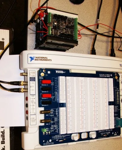
Input from frequency generator to filter
ELVIS II channel 0
Output from filter
ELVIS II channel 1
Figure 4: Part of equipment setup showing NI Elvis board
Results
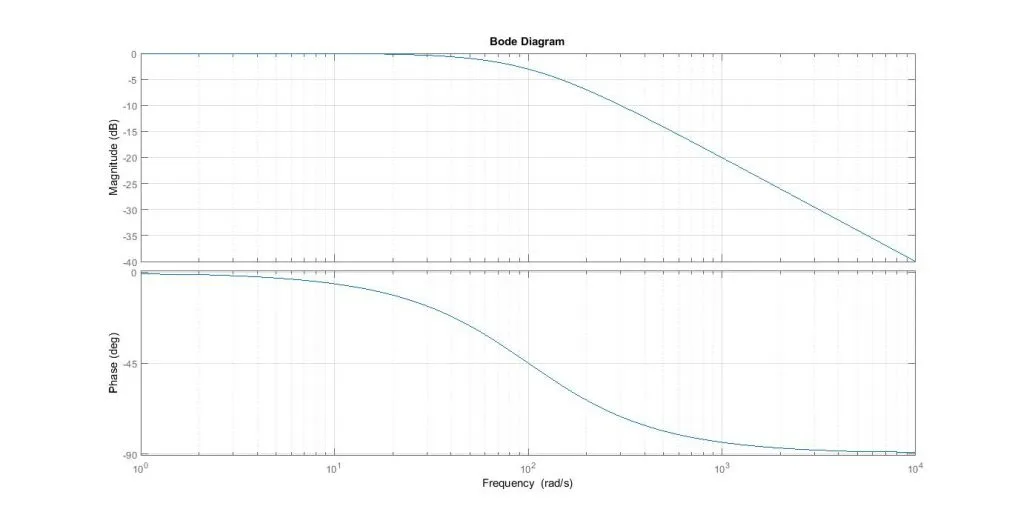
Figure 5: Bode plot when using a 100 k resistor
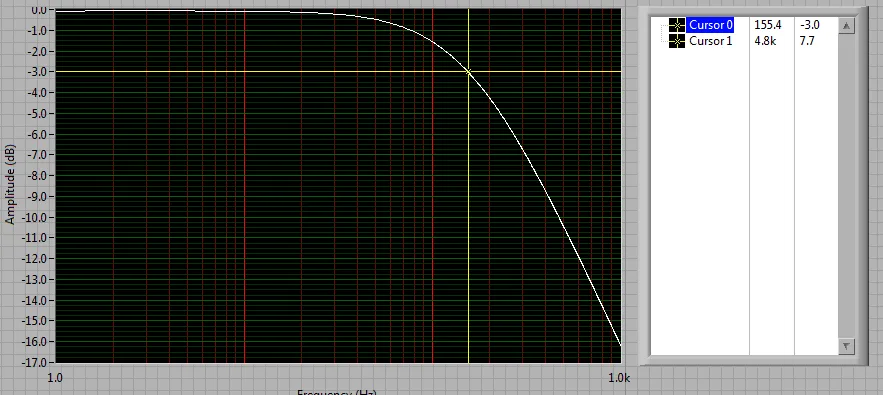
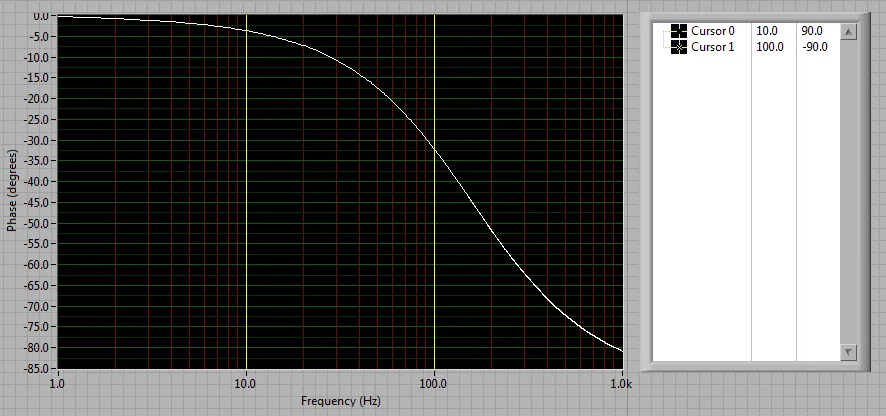
Figure 6: Bode plot for experimental data using 10k
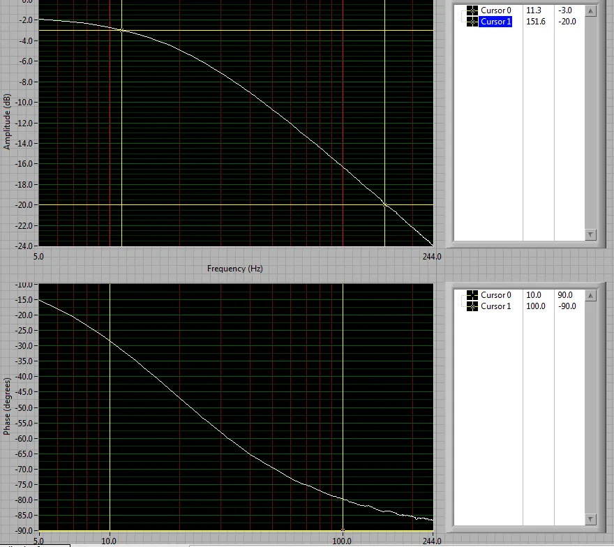
Figure 7: Bode plot for experimental data using 100 k
This section presents both theoretical results simulated in MATLAB and experimental results obtained from LabVIEW. The theoretical results for the circuit with a 10 k resistor in Figure (1) were presented earlier. When the resistance is increased to 100 k, the following calculations and MATLAB code were used:
MATLAB code:
num = [1000];
den = [1, 1000];
TF = tf(num,den)
bode(TF)
%TRANSFER FUNCTION:
100
s + 100
Figure (5) shows the resultant plot for the code used in MATLAB.
Figures (6) and (7) are the practical results for both 10 k and 100 k resistors, respectively.
Discussion
The theoretical curve from MATLAB and the Bode plot from actual measurement was indeed matching in both magnitude and phase for the various cases. The Bode plot shows the frequency response of both to be nearly flat in the lower frequencies; the result is that the output was almost the same as the input, that is, a gain close to unity is achieved until reaching the corner frequency; the latter being -3 dB or Vout = 0.707 Vin (Lascu, L., Boldea, & Blaabjerg, 2009). For higher frequencies, it gradually reduces for both magnitude and phase. The magnitude reduces at a rate of 20dB/decade while the phase eventually becomes -900. The explanation for this is that a capacitor has high capacitive reactance for lower frequencies and hence blocks the flow of current. On the other hand, for medium-high frequencies, the capacitor starts to conduct, acting as a typical short circuit for higher frequencies (Passive Low Pass Filter, 2016). Hence, the output voltage will be zero.
The effect of reducing the resistor in the RC circuit from 100 k to 10 k is that it raises the cut-off frequency from 16 HZ to 160 Hz, as shown by the equation below:
Cut-off frequency when R= 100 k:
Cut-off frequency when R= 10 k:
The effect of increasing the value of the capacitor from 0.1 μF to 1 μF while keeping the resistance at 100 k is that it reduces the cut-off frequency from 16 Hz to 1.6 Hz, as shown below:
The equation above shows that the capacitor is more sensitive; hence, a slight change in its value has a substantial effect on the circuit parameters. The implication of this is that by carefully choosing the desirable resistor and capacitor duo, an RC circuit that selectively allows or blocks a certain range of frequencies can be achieved (Miller, Outlaw, & Holloway, 2010). For this lab, the RC combination was operating as a first-order low-pass filter. Low pass filters only allow lower frequencies to pass while blocking higher frequencies. Other common filters used in analogue electronics are the high pass filter, band pass filter, and band stop filter (Sun, 2002).
Various possible sources of errors include contact losses, resistances in cable resulting in some losses, possibilities of trade-offs during plotting of Bode plot, and theoretical curves.
Conclusion
The lab session was a success, and the objective was fully met. The frequency response of RC circuits was explored. RC circuits can be used to make analogue filters. The test RC circuits used in the experiment were low-pass filters. A low pass filter selectively allows lower frequencies of an input signal to pass while blocking higher frequencies. The bandwidth of the filter is measured from zero to the cut-off frequency. The cut-off frequency is also known as the corner frequency and is usually at -3 dB of the input voltages.
References
Aparicio, R., & Hajimiri, A. (2002). Capacity limits and matching properties of integrated capacitors. IEEE Journal of Solid-State Circuits, 37(3), 384-393.
Lascu, C., L., A., Boldea, I., & Blaabjerg, F. (2009). Frequency response analysis of current controllers for selective harmonic compensation in active power filters. IEEE Transactions on Industrial Electronics, 56(2), 337-347.
Miller, J. R., Outlaw, R. A., & Holloway, B. C. (2010). Graphene double-layer capacitor with AC line-filtering performance. Science, 1637-1639.
Ni Elvis II. (2018, January). Retrieved from National Instruments: http://www.ni.com/en-za/support/model.ni-elvis-ii.html
Passive Low Pass Filter. (2016, January 15). Retrieved from Electronics-utorials: http://www.electronics-tutorials.ws/filter/filter_2.html
Sun, Y. (Ed.). (2002). Design of high frequency integrated analogue filters (No. 14). Iet.
Cite This Work
To export a reference to this article please select a referencing stye below: